x<-c(20,21,15,18,25)
(devx<-x-mean(x))
[1] 0.2 1.2 -4.8 -1.8 5.2Quantifying relationships between variables is an important skill in business analytics. The regression line, representing the best linear fit between two variables, enables businesses to make predictions, identify trends, and optimize strategies using data-driven insights. Understanding how to calculate and interpret a regression line provides the foundation for analyzing business relationships, such as the effect of advertising on sales or customer satisfaction on revenue. Below, we delve into generating and analyzing a regression line.
The regression line is calculated to minimize the average distance (or errors) between the line and the observed data points. It is defined by two key components: a slope (\(\hat{\beta}\)) and an intercept (\(\hat{\alpha}\)). Mathematically, the regression line is expressed as:
THE REGRESSION LINE \[\hat{y_i}=\hat{\alpha}+\hat{\beta}x_i\] where \(\hat{y_i}\) are the predicted values of \(y\) given \(x_i\), \(\hat{\alpha}\) is the intercept, and \(\hat{\beta}\) is the slope.
The slope determines the steepness of the line and quantifies how much a unit increase in \(x\) changes \(y\) on average. It is calculated using the covariance between \(y\) and \(x\) and the variance of \(x\):
THE SLOPE \[\hat{\beta}= \frac{s_{xy}}{s_{x}^2}\] where \(s_{xy}\) is the sample covariance between \(x\) and \(y\), and \(s_x^2\) is the sample variance of \(x\).
The intercept determines where the line crosses the \(y\) axis — the predicted value of \(y\) when \(x\) is zero. Once the slope is estimated, the intercept is calculated by:
THE INTERCEPT \[\hat{\alpha}=\bar{y}-\hat{\beta}\bar{x}\] where \(\bar{y}\) is the mean of \(y\) and \(\bar{x}\) is the mean of \(x\).
Example: Let’s examine a data set on Price and Advertisement. In general, one expects that when a company advertises, it can convince consumers to pay more for their product. Below is the data:
| Advertisement (x) | Price (y) |
|---|---|
| 2 | 7 |
| 1 | 3 |
| 3 | 8 |
| 4 | 10 |
The data shows a clear direct relationship between advertisement and price. Regression allows us to answer two key questions:
Step 1 — Calculate the slope: Given that the covariance is \(s_{xy}=3.67\) and the variance of \(x\) is \(s_x^2=1.67\):
\[\hat{\beta}= \frac{3.67}{1.67}=2.2\]
For every additional dollar spent on advertisement, price increases by \(2.2\) on average.
Step 2 — Calculate the intercept: Since \(\bar{x}=2.5\) and \(\bar{y}=7\):
\[\hat{\alpha}=7-2.2(2.5)=1.5\]
If we do not advertise, the predicted price is \(1.5\).
Step 3 — Write the regression line:
\[\hat{y_i}=1.5+2.2x_i\]
Step 4 — Make a prediction: With an advertisement budget of \(6\):
\[\hat{y_i}=1.5+2.2(6)=14.7\]
In conclusion, for every dollar spent on advertisement the price increases by \(2.2\), and with a budget of \(6\) the predicted price is \(14.7\).
When analyzing the effectiveness of a regression model, it is crucial to assess how well the model fits the data. Below we revisit the coefficient of determination \(R^2\) and introduce additional measures.
The coefficient of determination or \(R^2\) is the percent of the variation in \(y\) that is explained by changes in \(x\). The higher the \(R^2\) the better the explanatory power of the model.
THE COEFFICIENT OF DETERMINATION \[R^2=\frac{SSR}{SST}\]
where:
\(R^2\) is always between \([0,1]\).
Example: Consider data on the Weight (\(y\)) and Exercise (\(x\)) of a particular person:
| Weight (y) | Exercise (x) |
|---|---|
| 165 | 45 |
| 170 | 10 |
| 168 | 25 |
| 164 | 30 |
| 165 | 40 |
If we used only the mean \(\bar{y}=166.4\) as our prediction, the total squared error would be:
\[SST=(-1.4)^2+(3.6)^2+(1.6)^2+(-2.4)^2+(-1.4)^2=25.2\]
Using the regression line reduces these errors. The mistakes made by the regression line are quantified by:
\[SSE=0.81+0.29+0.69+5.76+0.02=7.57\]
The improvement gained by using regression over the mean is:
\[SSR=5.29+9.4+0.59+0+2.35=17.63\]
Hence the coefficient of determination is:
\[R^2=\frac{SSR}{SST}=\frac{17.63}{25.2}\approx0.70\]
The regression line explains about \(70\%\) of the variation in Weight using Exercise.
If we were to predict weight we could use several other variables to get a better prediction. Multiple regression is a technique used to predict a variable using more than one independent variable.
THE MULTIPLE REGRESSION LINE \[\hat{y_i}=\hat{\beta_0}+\hat{\beta_1}x_1+\hat{\beta_2}x_2+...+\hat{\beta_k}x_k\] where \(k\) is the total number of independent variables included in the model.
Example: Let’s consider an additional variable in our Weight and Exercise example. The table below includes information on Calories (\(z\)):
| Weight (y) | Exercise (x) | Calories (z) |
|---|---|---|
| 165 | 45 | 1200 |
| 170 | 10 | 1260 |
| 168 | 25 | 1220 |
| 164 | 30 | 1180 |
| 165 | 40 | 1190 |
The multiple regression line estimated by computer software is:
\[\hat{y_i}=83.96-0.025x+0.069z\]
Two conclusions follow from this result. First, as exercise increases weight tends to go down, while more calories increases weight. Second, reducing calorie consumption by \(1\) unit decreases weight by \(0.069\) pounds, whereas one additional minute of exercise only reduces weight by \(0.025\) pounds — making calorie reduction more effective per unit.
The Anova table helps us understand how well each variable in our regression model explains the dependent variable. It decomposes the \(SSR\) by variable and tracks the remaining errors.
Example: For the Weight, Exercise, and Calories regression, the Anova table is:
| Source | Sum Squares |
|---|---|
| x | 17.63 |
| z | 6.55 |
| Residuals | 1.01 |
Exercise explains \(17.63\) of the total variation. Adding Calories reduces the remaining unexplained variation by another \(6.55\), bringing the total \(SSR\) to \(24.18\) and the \(SSE\) down to \(1.01\). The \(R^2\) increases from \(0.70\) to:
\[R^2=\frac{17.63+6.55}{25.2}=0.96\]
The adjusted \(R^2\) penalizes a model for including additional explanatory variables, preventing artificial inflation of \(R^2\).
THE ADJUSTED \(R^2\) \[\bar{R}^2=1-(1-R^2)\frac{n-1}{n-k-1}\] where \(k\) is the number of explanatory variables and \(n\) is the sample size.
Example: For the Weight example with both Exercise and Calories (\(k=2\), \(n=5\), \(R^2=0.96\)):
\[\bar{R}^2=1-(1-0.96)\frac{5-1}{5-2-1}=0.92\]
The Residual Standard Error estimates the average dispersion of the data points around the regression line.
THE RESIDUAL STANDARD ERROR \[s_e=\sqrt{\frac{SSE}{n-k-1}}\] where \(k\) is the number of independent variables and \(n\) is the sample size.
Example: For the Weight and Exercise model (\(k=1\)):
\[s_e=\sqrt{\frac{7.57}{5-1-1}}=1.59\]
Adding Calories (\(k=2\)) reduces this to:
\[s_e=\sqrt{\frac{1.01}{5-2-1}}=0.71\]
The smaller residual standard error confirms that adding Calories improves the model’s fit.
Excel provides a straightforward way to estimate regression models using the Data Analysis ToolPak. If it is not already enabled, go to File → Options → Add-ins → Analysis ToolPak → Go and check the box.
Simple Regression (Weight and Exercise):
Data → Data Analysis → RegressionOKExcel will produce a full regression output including the coefficients, \(R^2\), Adjusted \(R^2\), Standard Error, and Anova table — all in one step.
Reading the Excel Output:
Multiple Regression (Weight, Exercise, and Calories):
Follow the same steps but set the Input X Range to include both the Exercise and Calories columns. Excel handles multiple predictors automatically.
Making Predictions: Once you have the coefficients from the output, use them directly in a formula. For the Advertisement and Price example, if the intercept is in cell B17 and slope in B18:
=B17 + B18 * 6This returns the predicted price for an advertisement budget of \(6\).
Below is a list of the Excel functions and tools used in this section:
Data Analysis ToolPak → Regression is the primary tool for estimating regression models in Excel. It returns coefficients, \(R^2\), adjusted \(R^2\), standard error, and the Anova table in a single output.
=SLOPE(y_range, x_range) calculates the slope \(\hat{\beta}\) of the simple regression line directly.
=INTERCEPT(y_range, x_range) calculates the intercept \(\hat{\alpha}\) of the simple regression line directly.
=FORECAST.LINEAR(x, y_range, x_range) returns the predicted value of \(y\) for a given value of \(x\) using simple linear regression.
=RSQ(y_range, x_range) returns the \(R^2\) for a simple regression.
=STEYX(y_range, x_range) returns the residual standard error \(s_e\) for a simple regression.
The following exercises will help you get practice on Regression Line estimation and interpretation. In particular, the exercises work on:
Answers are provided below. Try not to peak until you have formulated your own answer and double checked your work for any mistakes.
For the following exercises, make your calculations by hand and verify results using R functions when possible.
| x | 20 | 21 | 15 | 18 | 25 |
|---|---|---|---|---|---|
| y | 17 | 19 | 12 | 13 | 22 |
The regression lines is \(\hat{y}=-4.93+1.09x\). For each unit increase in x, y increases on average \(1.09\).
Start by generating the deviations from the mean for each variable. For x the deviations are:
x<-c(20,21,15,18,25)
(devx<-x-mean(x))[1] 0.2 1.2 -4.8 -1.8 5.2Next, find the deviations for y:
y<-c(17,19,12,13,22)
(devy<-y-mean(y))
[1] 0.4 2.4 -4.6 -3.6 5.4For the slope we need to find the deviation squared of the x’s. This can easily be done in R:
(devx2<-devx^2)[1] 0.04 1.44 23.04 3.24 27.04The slope is calculated by \(\frac{\sum_{i=i}^{n}(x_{i}-\bar{x})(y_{i}-\bar{y})}{\sum_{i=i}^{n}(x_{i}-\bar{x})^2}\). In R we can just find the ratio between the summations of (devx)(devy) and devx2.
(slope<-sum(devx*devy)/sum(devx2))[1] 1.087591The intercept is given by \(\bar{y}-\beta(\bar{x})\). In R we find that the intercept is equal to:
(intercept<-mean(y)-slope*mean(x))[1] -4.934307Our results can be easily verified by using the lm() and coef() functions in R.
fitEx1<-lm(y~x)
coef(fitEx1)
(Intercept) x
-4.934307 1.087591 SST is \(69.2\), SSR is \(64.82\) and SSE is \(4.38\) (note that \(SSR+SSE=SST\)). The \(R^2\) is just \(\frac{SSR}{SST}=0.94\) and the Standard Error estimate is \(1.21\). They both indicate a great fit of the regression line to the data.
Let’s start by calculating the SST. This is just \(\sum{(y_{i}-\bar{y})^2}\).
(SST<-sum((y-mean(y))^2))[1] 69.2Next, we can calculate SSR. This is calculated by the following formula \(\sum{(\hat{y_{i}}-\bar{y})^2}\). To obtain the predicted values in R, we can use the output of the lm() function. Recall our fitEx1 object created in Exercise 1. It has fitted.values included:
(SSR<-sum((fitEx1$fitted.values-mean(y))^2))[1] 64.82044The ratio of SSR to SST is the \(R^2\):
(R2<-SSR/SST)[1] 0.9367115Finally, let’s calculate SSE \(\sum{(y_{i}-\hat{y_{i}})^2}\):
(SSE<-sum((y-fitEx1$fitted.values)^2))[1] 4.379562With the SSE we can calculate the Standard Error estimate:
sqrt(SSE/3)[1] 1.208244We can confirm these results using the summary() function.
summary(fitEx1)
Call:
lm(formula = y ~ x)

Residuals:
      1       2       3       4       5
 0.1825  1.0949  0.6204 -1.6423 -0.2555

Coefficients:
            Estimate Std. Error t value Pr(>|t|)
(Intercept)  -4.9343     3.2766  -1.506  0.22916
x             1.0876     0.1632   6.663  0.00689 **
---
Signif. codes:  0 '***' 0.001 '**' 0.01 '*' 0.05 '.' 0.1 ' ' 1

Residual standard error: 1.208 on 3 degrees of freedom
Multiple R-squared:  0.9367,    Adjusted R-squared:  0.9156
F-statistic: 44.4 on 1 and 3 DF, p-value: 0.00689If \(x=32\) then \(\hat{y}=29.87\). The regression is a good fit, so we can feel good about our prediction. However, we would be concerned about the sample size of the data.
In R we can obtain a prediction by using the predict() function. This function requires a data frame as an input for new data.
predict(fitEx1, newdata = data.frame(x=c(32))) 1
29.86861 You will need the Education data set to answer this question. You can find the data set at https://jagelves.github.io/Data/Education.csv . The data shows the years of education (Education), and annual salary in thousands (Salary) for a sample of \(100\) people.
An extra year of education increases the annual salary about \(5,300\) dollars (slope). A person that has no education would be expected to earn \(17,258\) dollars (intercept).
Start by loading the data in R:
library(tidyverse)
Education<-read_csv("https://jagelves.github.io/Data/Education.csv")
Next, let’s use the lm() function to estimate the regression line and obtain the coefficients:
fitEducation<-lm(Salary~Education, data = Education)
coefficients(fitEducation)
(Intercept) Education
17.258190 5.301149 The \(R^2\) is \(0.668\) and the standard error is \(21\). The line is a moderately good fit. If someone has \(16\) years of education, the regression line would predict a salary of \(102,000\) dollars.
Let’s get the \(R^2\) and the Standard Error estimate by using the summary() function and fitEducation object.
summary(fitEducation)
Call:
lm(formula = Salary ~ Education, data = Education)

Residuals:
    Min      1Q  Median      3Q     Max
-62.177  -9.548   1.988  15.330  45.444

Coefficients:
            Estimate Std. Error t value Pr(>|t|)
(Intercept)  17.2582     4.0768   4.233  5.2e-05 ***
Education     5.3011     0.3751  14.134  < 2e-16 ***
---
Signif. codes:  0 '***' 0.001 '**' 0.01 '*' 0.05 '.' 0.1 ' ' 1

Residual standard error: 20.98 on 98 degrees of freedom
Multiple R-squared:  0.6709,    Adjusted R-squared:  0.6675
F-statistic: 199.8 on 1 and 98 DF,  p-value: < 2.2e-16
Lastly, let’s use the regression line to predict the salary for someone who has \(16\) years of education.
predict(fitEducation, newdata = data.frame(Education=c(16))) 1
102.0766 You will need the FoodSpend data set to answer this question. You can find this data set at https://jagelves.github.io/Data/FoodSpend.csv .
Approximately, \(36\)% of the sample owns a home.
Start by loading the data into R and removing all NA’s:
Spend<-read_csv("https://jagelves.github.io/Data/FoodSpend.csv")Rows: 80 Columns: 2
── Column specification ────────────────────────────────────────────────────────
Delimiter: ","
chr (1): OwnHome
dbl (1): Food
ℹ Use `spec()` to retrieve the full column specification for this data.
ℹ Specify the column types or set `show_col_types = FALSE` to quiet this message.Spend<-na.omit(Spend)To create a dummy variable for OwnHome we can use the ifelse() function:
Spend$dummyOH<-ifelse(Spend$OwnHome=="Yes",1,0)The average of the dummy variable is given by:
mean(Spend$dummyOH)[1] 0.3625The intercept is the average food expenditure of individuals without homes (\(6417\)). The slope is the difference in food expenditures between individuals that do have homes minus those who don’t. Individuals that do have a home spend about \(-2516\) less on food than those who don’t have homes.
To run the regression use the lm() function:
lm(Food~dummyOH,data=Spend)
Call:
lm(formula = Food ~ dummyOH, data = Spend)

Coefficients:
(Intercept)      dummyOH
6473 -3418 The scatter plot shows that most of the points for home owners are below \(6000\). For non-home owners they are mainly above \(6000\). The line can be used to predict the likelihood of owning a home given someone’s food expenditure. The slope tells us how that likelihood changes as the food expenditure increases by 1 — in general, the likelihood of owning a home decreases as food expenditure increases.
Run the lm() function once again:
fitFood<-lm(dummyOH~Food,data=Spend)
coefficients(fitFood)
(Intercept) Food
1.4320766616 -0.0002043632 For the scatter plot use the following code:
library(ggthemes)
Spend %>% ggplot() +
  geom_point(aes(y=dummyOH,x=Food),
             col="black", pch=21, bg="grey") +
  geom_smooth(aes(y=dummyOH,x=Food), method="lm",
              formula=y~x, se=F) +
  theme_clean()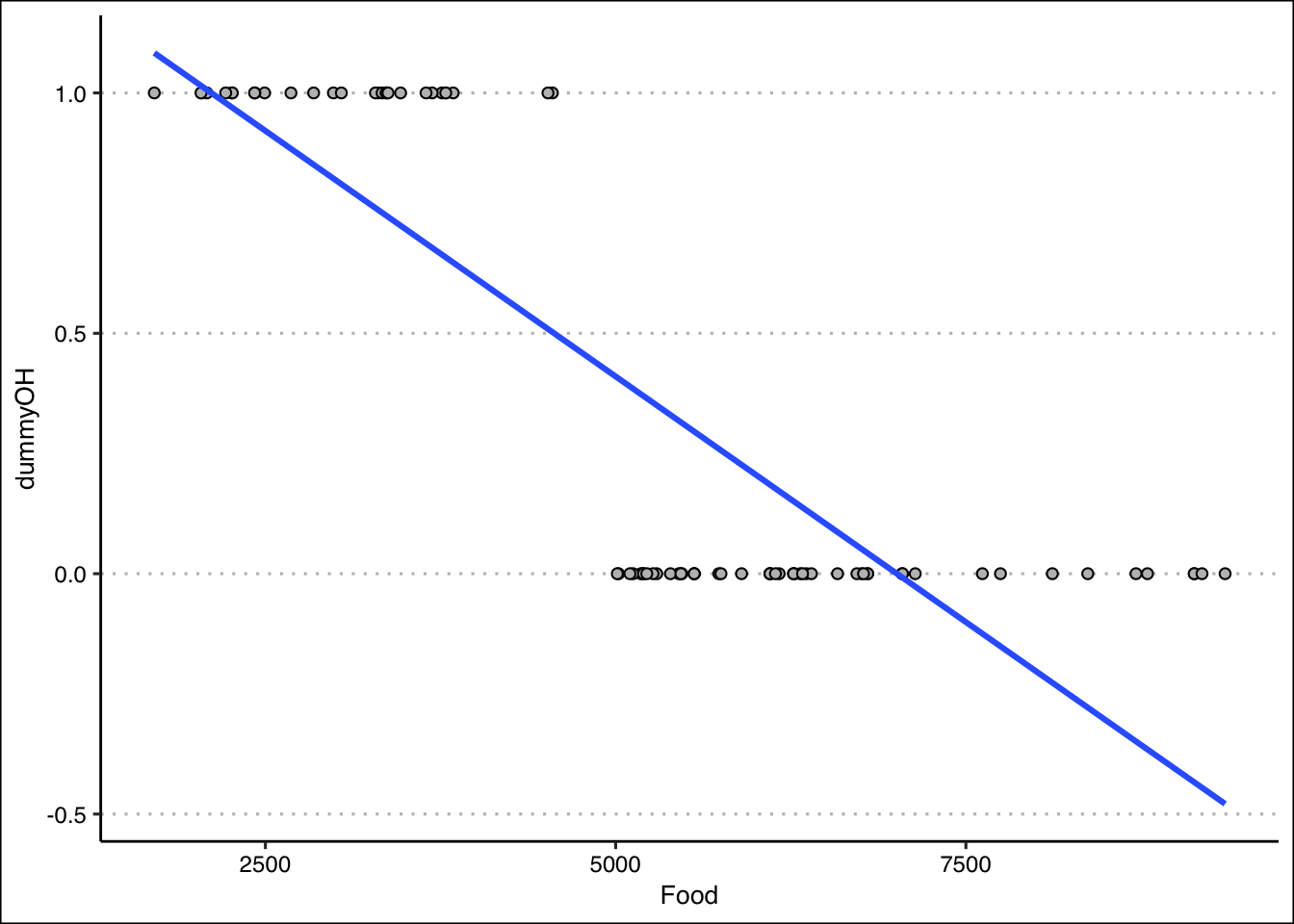
You will need the Population data set to answer this question. You can find this data set at https://jagelves.github.io/Data/Population.csv .
If we follow the \(R^2=0.81\) the model fits the data very well.
Let’s load the data from the web:
Population<-read_csv("https://jagelves.github.io/Data/Population.csv")New names:
Rows: 16492 Columns: 4
── Column specification
──────────────────────────────────────────────────────── Delimiter: "," chr
(1): Country.Name dbl (3): ...1, Year, Population
ℹ Use `spec()` to retrieve the full column specification for this data. ℹ
Specify the column types or set `show_col_types = FALSE` to quiet this message.
• `` -> `...1`Now let’s filter the data so that we can focus on the population for Japan.
Japan<-filter(Population,Country.Name=="Japan")Next, we can run the regression of Population against the Year. Let’s also run the summary() function to obtain the fit and the coefficients.
fit<-lm(Population~Year,data=Japan)
summary(fit)
Call:
lm(formula = Population ~ Year, data = Japan)

Residuals:
     Min       1Q   Median       3Q      Max
-9583497 -4625571  1214644  4376784  5706004

Coefficients:
              Estimate Std. Error t value Pr(>|t|)
(Intercept) -988297581   68811582  -14.36   <2e-16 ***
Year            555944      34569   16.08   <2e-16 ***
---
Signif. codes:  0 '***' 0.001 '**' 0.01 '*' 0.05 '.' 0.1 ' ' 1

Residual standard error: 4871000 on 60 degrees of freedom
Multiple R-squared:  0.8117,    Adjusted R-squared:  0.8086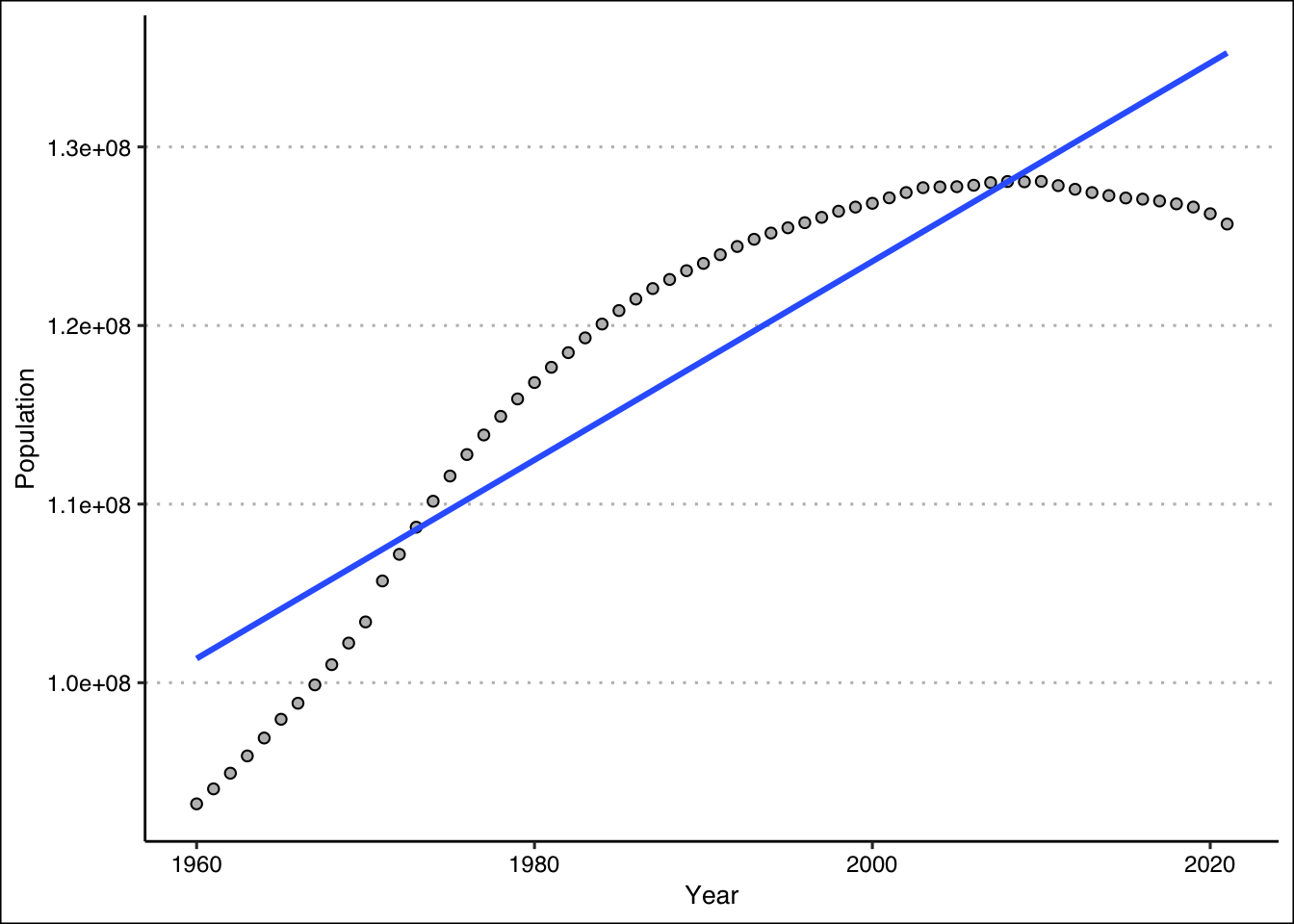
F-statistic: 258.6 on 1 and 60 DF, p-value: < 2.2e-16The prediction for \(2030\) is about \(140\) million people.
Let’s use the predict() function:
predict(fit,newdata=data.frame(Year=c(2030))) 1
140268585 After looking at the scatter plot, it seems unlikely that the population in Japan will hit \(140\) million. Population has been decreasing in Japan!
Use ggplot to create the figure.
Japan %>% ggplot() +
  geom_point(aes(y=Population,x=Year),
             col="black", pch=21, bg="grey") +
  geom_smooth(aes(y=Population,x=Year),
              formula=y~x, method="lm", se=F) +
  theme_clean()