| Date | People | Approval |
|---|---|---|
| 01/01/24 | 50 | 25% |
| 02/01/24 | 100 | 25% |
| 03/01/24 | 30 | 70% |
| 04/01/24 | 250 | 85% |
3 Descriptive Statistics III
Understanding where the “center” of a dataset lies is a fundamental step when interpreting and analyzing data. Measures of central location provide different ways to identify the “typical” value in a dataset, each with its unique strengths and limitations. Below I survey some of the most popular measures of central location. These summaries continue the work of describing our data: having seen its overall shape, we now pin down its center — a single representative value that will later anchor the estimates we carry into inference.
3.1 Sample Vs. Population Statistics
In this book you will find formulas for calculating sample statistics and population parameters. In general, you will use population formulas when you have data for the entire group you care about or when you are working with a theoretical distribution and the parameter is known; population formulas use \(N\) in denominators and estimate parameters. Use sample formulas when your data are a subset drawn from a larger population and you want unbiased estimators of the population parameters; sample formulas use \(n\) and the degrees of freedom correction. In practice most empirical work uses sample formulas because we rarely observe entire populations; below you will see both population and sample versions so you can choose the correct one depending on whether your data represent the full population or a sample.
3.2 The Mean
The mean is the average value for a numerical variable. It is a widely understood and straightforward measure to calculate. It incorporates all data points, providing a comprehensive representation of the data set. However, its reliance on every value also makes it sensitive to outliers or skewed distributions, which may cause it to not accurately reflect the true center of the data.
The sample statistic is estimated by:
THE MEAN (Sample) \[\bar{x}=\frac{\sum x_{i}}{n}\]
where \(\Sigma\) is the summation operator, \(x_i\) is observation \(i\), and \(n\) is the number of observations in the sample.
The formula instructs you to add up all of the values in a variable and then divide by the sample size. If you wish to estimate the population parameter you can use:
THE MEAN (Population) \[\mu=\frac{\sum x_{i}}{N}\]
where \(N\) is the population size.
Let’s consider a couple of example to highlight how the formula works.
Example 1: Consider the following sample of numbers \(x=\{1,4,2,1\}\). The mean would be equal to \(\bar{x}=\frac{1+4+2+1}{4}\) or \(\bar{x}=2\).
Example 2: Consider the following sample of numbers \(x=\{1,4,2,1,100\}\). The mean is \(\bar{x}=21.6\). Although most of the numbers are in the range \((1,4)\), the \(100\) biases the mean to \(21.6\).
3.3 The Median
The median is the value in the middle when data is organized in ascending order. When \(n\) is even, the median is the average between the two middle values. The median is resistant to outliers, making it an ideal measure for skewed data or data sets with irregular distributions. It is particularly useful for ordinal data, where precise ranking is important. However, the median does not utilize all data points, which can lead to less precise comparisons compared to other measures like the mean.
Example 1: Consider the following numbers \(x=\{1,4,2,1\}\). We first sort the data to obtain \(x_{sorted}=\{1,1,2,4\}\). Since the number of observations is even (\(n=4\)), the median is the average of the two middle numbers \((1,2)\). \(median_x=\frac{1+2}{2}\) or \(1.5\).
Example 2: Consider the following numbers \(x=\{1,4,2,1,100\}\). We once again sort the number obtaining \(x_{sorted}=\{1,1,2,4,100\}\). Since \(n=5\) in this case we can identify the median as the third value in \(x_{sorted}\). \(median_x=2\). Note that the inclusion of \(100\) in the data did not change much the measure of central location.
3.4 The Mode
The mode is the value with highest frequency from a set of observations. This measure is particularly useful for categorical data as it helps determine popularity of values. It can be applied to both numerical and non-numerical data sets. The mode has its limitations; it may not exist in cases where all values occur with equal frequency, and there may be multiple modes, which can complicate interpretation. Additionally, since the mode focuses only on the most frequent value, it does not account for other data points, limiting its overall utility as a comprehensive measure.
Example 1: Consider the following numbers \(x=\{1,4,2,1\}\). Since \(1\) is repeated twice and all other numbers just repeated once, \(x_{mode}=1\).
Example 2: Consider the following numbers \(x=\{1,4,2,1,4\}\). Now \(4\) is also repeated twice. The variable has two modes \(x_{mode}=\{1,2\}\). \(x\) is said to be bimodal.
3.5 The Weighted Mean
The weighted mean is useful in scenarios where some data points are more significant than others, such as in financial portfolios, grade point averages, or survey results, as it accounts for variability in importance across observations. This measure requires additional information in the form of weights (\(w_i\)), which may not always be available or accurate. It is calculated the sum product of values (\(x_i\)) and weights (\(w_i\)) and then dividing by the sum of weights. Mathematically, the weighted average is:
THE WEIGHTED MEAN \[\bar{x}_w=\frac{\sum w_{i}x_{i}}{\sum w_{i}}\] where \(w_{i}\) represents the weight of the ith observation.
Let’s consider once more a couple of examples.
Example 1: Consider three different stocks \(S=\{T, C, X\}\) with stock returns of \(R=\{2,4,10\}\). Each stock has a weight in the portfolio of \(W=\{0.3,0.2,0.5\}\). The average return of the portfolio is \(\bar{x}_{weighted}=\frac{0.6+0.8+5}{1}\) or \(\bar{x}_{weighted}=6.4\).
Example 2: A company evaluates job candidates using three criteria: technical skills, communication, and teamwork. The criteria and their weights are shown in the table below:
| Criteria | Weight | Score |
|---|---|---|
| Technical Skills | 0.50 | 88 |
| Communication | 0.30 | 76 |
| Teamwork | 0.20 | 82 |
The weighted mean score for the candidate is:
\[\bar{x}_w = (0.50 \times 88) + (0.30 \times 76) + (0.20 \times 82)\]
\[= 44 + 22.8 + 16.4 = 83.2\]
The candidate’s overall score is \(83.2\) out of \(100\). Note that a simple average would have given \((88 + 76 + 82)/3 = 82\), a slightly different result. The weighted mean reflects the company’s priorities by giving more importance to technical skills.
3.6 The Geometric Mean
The geometric mean is a multiplicative average that is less sensitive to outliers relative to the arithmetic mean. It is particularly useful when averaging rates or levels that compound over time. The formula depends on whether the data represents rates or levels.
When working with rates, we add 1 to each value because rates represent changes relative to a base value. The geometric mean is given by:
THE GEOMETRIC MEAN (Rates) \[\bar{x}_g=\sqrt[n]{(1+r_1)\times(1+r_2)\times...\times(1+r_n)}-1\] where \(r_i\) are rates of change and \(n\) is the number of periods.
When working with levels, the values already reflect standalone quantities rather than relative changes, so no adjustment is needed. The geometric mean simplifies to:
THE GEOMETRIC MEAN (Levels) \[\bar{x}_g=\sqrt[n]{x_1 \times x_2 \times ... \times x_n}\] where \(x_i\) are positive values such as prices, proportions, or index values.
To illustrate the distinction, we work through two examples below.
Example 1: A company tracks its market share across four regions: \(x=\{0.20, 0.30, 0.10, 0.10\}\). Since market share is a proportion of the whole — a level, not a rate of change — we apply the levels formula directly:
\[\bar{x}_g=\sqrt[4]{0.20 \times 0.30 \times 0.10 \times 0.10}\] \[=\sqrt[4]{0.0006}=0.156\]
The geometric mean market share across the four regions is \(15.6\%\).
Example 2: An investment fund reports the following annual returns over four years:
| Year | Return | Growth Factor |
|---|---|---|
| 2020 | 10% | 1.10 |
| 2021 | 25% | 1.25 |
| 2022 | -8% | 0.92 |
| 2023 | 15% | 1.15 |
Since these are rates of return, we add 1 to each value to obtain the growth factor before applying the formula. The geometric mean is:
\[\bar{x}_g = \sqrt[4]{1.10 \times 1.25 \times 0.92 \times 1.15}-1\] \[= \sqrt[4]{1.4539}-1 = 0.0977\]
The average annual return is \(9.77\%\). Note that the arithmetic mean gives \((10 + 25 - 8 + 15)/4 = 10.5\%\), which overstates the true average. The geometric mean is the appropriate measure here because it accounts for the compounding effect of returns over time.
3.7 Measures of Central Location in Excel
Excel has a collection of functions that calculate measures of central location. Let’s consider the following data on approval ratings:
You can also download the data here:
Mean: To calculate the mean in Excel use =AVERAGE(C2:C5), where column C contains the approval ratings. The mean approval rating is 0.5125.
Median: To calculate the median in Excel use =MEDIAN(C2:C5). The median approval rating is 0.475.
Mode: To calculate the mode in Excel use =MODE(C2:C5). Note that MODE only returns one value even if there are multiple modes. For the approval data, the mode is 0.25.
Weighted Mean: To calculate the weighted mean in Excel use =SUMPRODUCT(B2:B5, C2:C5) / SUM(B2:B5), where column B contains the number of people surveyed and column C contains the approval ratings. This formula multiplies each approval rating by its corresponding weight and divides by the total number of people. The weighted mean approval rating is 0.6302326.
Geometric Mean: To calculate the geometric mean in Excel use =GEOMEAN(C2:C5). Note that since approval ratings are already proportions there is no need to add 1 to each value before applying the formula. The geometric mean approval rating is 0.4391.
3.8 Excel Function Summary
=AVERAGE()calculates the mean for a range of numbers.=MEDIAN()calculates the median for a range of numbers.=MODE()returns the most frequently occurring value in a range.=SUMPRODUCT()multiplies corresponding values in two ranges and returns their sum, useful for calculating the weighted mean.=GEOMEAN()calculates the geometric mean for a range of numbers.
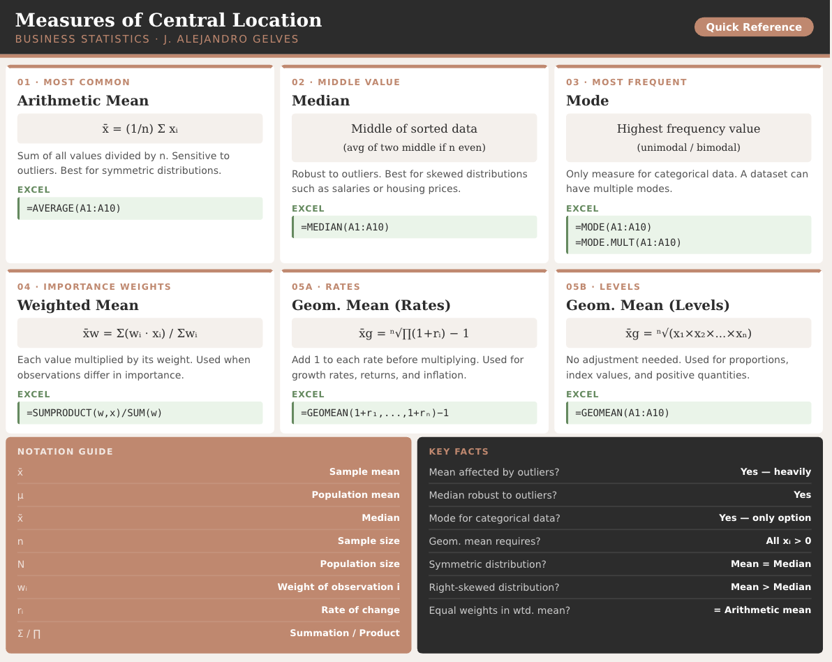
3.9 Chapter Summary Cheat Sheet
3.10 Exercises
The following exercises will help you practice the measures of central location. In particular, the exercises work on:
Calculating the mean, median, and the mode.
Calculating the weighted average.
Applying the geometric mean for growth rates and returns.
Answers are provided below. Try not to peek until you have a formulated your own answer and double checked your work for any mistakes.
Exercise 1
For the following exercises, make your calculations by hand and verify results using Excel functions when possible.
Use the following observations to calculate the mean, the median, and the mode.
8 10 9 12 12
Answer
To find the mean we will use the following formula \(( \frac{1}{n} \sum_{i=i}^{n} x_{i})\). The summation of the values is \(51\) and the number of observations is \(5\). The mean is \(51/5=10.2\).
The median is found by locating the middle value when data is sorted in ascending order. \(x_{sorted}=[8,9,10,12,12]\). The median in this example is \(10\).
The mode is the value with the highest frequency. In this example the mode is \(12\) since it is repeated twice and all other numbers appear only once.
To verify in Excel, enter the data in cells A1:A5 and use:
=AVERAGE(8,9,10,12,12)→ \(10.2\)=MEDIAN(8,9,10,12,12)→ \(10\)=MODE(8,9,10,12,12)→ \(12\)
Use following observations to calculate the mean, the median, and the mode.
-4 0 -6 1 -3 -4
Answer
The mean is \(-2.67\), the median is \(-3.5\), the mode is \(-4\). To verify in Excel, enter the data in cells A1:A6 and use:
=AVERAGE(-4,0,-6,1,-3,-4)→ \(-2.67\)=MEDIAN(-4,0,-6,1,-3,-4)→ \(-3.5\)=MODE(-4,0,-6,1,-3,-4)→ \(-4\)
Use the following observations, calculate the mean, the median, and the mode.
20 15 25 20 10 15 25 20 15
Answer
The mean is \(18.33\), the median is \(20\), the data is bimodal with both \(15\) and \(20\) being modes.
To verify in Excel, enter the data in cells A1:A9 and use:
=AVERAGE(20,15,25,20,10,15,25,20,15)→ \(18.33\)=MEDIAN(20,15,25,20,10,15,25,20,15)→ \(20\)=MODE.MULT(20,15,25,20,10,15,25,20,15)→ \(15\) and \(20\) (note: useMODE.MULTinstead ofMODEto capture all modes)
Exercise 2
You will need the OJ data set to answer this question. You can get the dataset here:
- Find the mean price for Country Hill (PriceCH) and Minute Maid (PriceMM).
Answer
The mean price for Country Hill is \(1.87\). The mean price for Minute Maid is \(2.09\).
To verify in Excel, assuming PriceCH is in column D and PriceMM is in column E, use:
=AVERAGE(D2:D1071)→ \(1.87\)=AVERAGE(E2:E1071)→ \(2.09\)
- Find the mean price of Country Hill (PriceCH) at each store (StoreID). Which store provides the better price?
Answer
The mean price at store 1 for Country Hill is \(1.80\). The juice is cheaper at store 1.The mean price at each store is:
# A tibble: 5 × 2
  StoreID MeanCH
    <dbl>  <dbl>
1       1   1.80
2       2   1.84
3       3   1.93
4       4   1.95
5       7   1.84
To verify in Excel, use AVERAGEIF to filter by store. Assuming StoreID is in column C and PriceCH is in column D:
=AVERAGEIF(C2:C1071, 1, D2:D1071)→ store 1 mean=AVERAGEIF(C2:C1071, 2, D2:D1071)→ store 2 mean=AVERAGEIF(C2:C1071, 3, D2:D1071)→ store 3 mean
- Find the median price paid by Country Hill (PriceCH) purchasers (Purchase) in all stores? Which store had the better median price?
Answer
Purchasers of Country Hill at store 1 paid a median price of \(1.76\) for Country Hill juice. This once again was the lowest price.The median price for Country Hill purchasers at each store is given by:
# A tibble: 5 × 2
  StoreID MedianCH
    <dbl>    <dbl>
1       1     1.76
2       2     1.86
3       3     1.99
4       4     1.99
5       7     1.86
To verify in Excel, use MEDIAN with IF as an array formula. Assuming Purchase is in column A, StoreID in column C, and PriceCH in column D. Enter with Ctrl+Shift+Enter:
=MEDIAN(IF((C2:C1071=1)*(A2:A1071="CH"), D2:D1071))→ store 1 median
Repeat changing the store number for each store.
Exercise 3
- Over the past year an investor bought TSLA. She made these purchases on three occasions at the prices shown in the table below. Calculate the average price per share.
| Date | Price Per Share | Number of Shares |
|---|---|---|
| February | 250.34 | 80 |
| April | 234.59 | 120 |
| Aug | 270.45 | 50 |
Answer
The average price of sale is found by using the weighted average formula. \(\frac{\sum w_{i}x_{i}}{\sum w_{i}}\) The weights (\(w_{i}\)) are given by the number of shares bought and the values (\(x_{i}\)) are the prices. The weighted average is \(246.802\).
To verify in Excel use:
=SUMPRODUCT({250.34,234.59,270.45},{80,120,50}) / SUM(80,120,50)→ \(246.802\)
- What would have been the average price per share if the investor would have bought equal amounts of shares each month?
Answer
The average if equal shares were bought would be \(251.7933\).
=AVERAGE(250.34,234.59,270.45)→ \(251.793\)
Exercise 4
Consider the following observations for the consumer price index (CPI). Calculate the inflation rate (Growth Rate of the CPI) for each period.
1 2 3 4 5 1.0 1.3 1.6 1.8 2.1
Answer
The inflation rate is the percentage change in the CPI. The inflation rate for each period is shown in the table below:
| 1-2 | 2-3 | 3-4 | 4-5 |
|---|---|---|---|
| 30% | 23.08% | 12.5% | 16.67% |
- What is the average growth rate for the inflation rate?
Answer
*The average growth rate is \(20.38%\). Use the geometric mean formula with compounding.
\[\bar x_{g}=(1.3 \times 1.2308 \times 1.125 \times 1.1667)^{1/4}-1\] \[\bar x_{g}=0.2038\]
You can use the command GEOMEAN(1.3,1.2308,1.125,1.1667)-1 in Excel to verify the result.
Exercise 5
Suppose that you want to invest $1000 dollars in a stock that is predicted to yield the following returns in the next four years. Calculate both the arithmetic mean and the geometric mean. Use the geometric mean to estimate how much money you would have by the end of year 4.
| Year | Annual Return |
|---|---|
| 1 | 17.3 |
| 2 | 19.6 |
| 3 | 6.8 |
| 4 | 8.2 |
Answer
At the end of 4 years it is predicted that you would have \(1621.17\) dollars. Each year you would have gained \(12.84\)% on average.
To verify in Excel use:
=AVERAGE(0.173, 0.196, 0.068, 0.082)→ \(0.12975\) arithmetic mean=GEOMEAN(1.173, 1.196, 1.068, 1.082)-1→ \(0.1173\) geometric mean=1000*(1+0.1173)^4→ \(1621.17\)
Exercise 6
You will need the Hitters dataset containing data on Major League Baseball players, including their salaries (in thousands of dollars) from 1987. You can get the dataset here:
- Compute the overall mean and median salary for all players. Which measure (mean or median) better represents the typical salary?
Answer
The mean and the median salary of the hitters is 535 and 425 respectively.Due to right-skew from superstar salaries, the median better represents the typical player.
To verify in Excel, assuming salaries are in column S, use:
=AVERAGE(S2:S323)→ \(535\)=MEDIAN(S2:S323)→ \(425\)
- filter to only players with at least one home run (HmRun >= 1) and compute the mean and median salary for this subgroup.
Answer
For players with ≥1 home run: mean higher (around 600+), median still lower than mean — skewness persists, median again more representative.
To verify in Excel, assuming salaries are in column S and home runs in column C:
=AVERAGEIF(C2:C323, ">=1", S2:S323)→ mean salary=MEDIAN(IF(C2:C323>=1, S2:S323))→ median salary