x<-c(20,21,15,18,25)
(devx<-x-mean(x))
[1] 0.2 1.2 -4.8 -1.8 5.2The regression line is fitted so that the average distance between the line and the sample points is as small as possible. The line is defined by a slope (\(\beta\)) and an intercept (\(\alpha\)). Mathematically, the regression line is expressed as \(\hat{y_i}=\hat{\alpha}+\hat{\beta}x_i\), where \(\hat{y_i}\) are the predicted values of \(y\) given the \(x\)’s.
The slope determines the steepness of the line. The estimate quantifies how much a unit increase in \(x\) changes \(y\). The estimate is given by \(\hat{\beta}= \frac {s_{xy}}{s_{x}^2}\).
The intercept determines where the line crosses the \(y\) axis. It returns the value of \(y\) when \(x\) is zero. The estimate is given by \(\hat{\alpha}=\bar{y}-\hat{\beta}\bar{x}\).
There are a couple of popular measures that determine the goodness of fit of the regression line.
The coefficient of determination or \(R^2\) is the percent of the variation in \(y\) that is explained by changes in \(x\). The higher the \(R^2\) the better the explanatory power of the model. The \(R^2\) is always between [0,1]. To calculate use \(R^2=SSR/SST\).
\(SSR\) (Sum of Squares due to Regression) is the part of the variation in \(y\) explained by the model. Mathematically, \(SSR=\sum{(\hat{y_i}-\bar{y})^2}\).
\(SSE\) (Sum of Squares due to Error) is the part of the variation in \(y\) that is unexplained by the model. Mathematically, \(SSE=\sum{(y_i-\hat{y_i})^2}\).
SST (Sum of Squares Total) is the total variation of \(y\) with respect to the mean. Mathematically, \(SST=\sum{(y_i-\bar{y})^2}\).
Note that \(SST=SSR+SSE\).
The adjusted \(R^2\) recognizes that the \(R^2\) is a non-decreasing function of the number of explanatory variables in the model. This metric penalizes a model with more explanatory variables relative to a simpler model. It is calculated by \(1-(1-R^2) \frac {n-1}{n-k-1}\), where \(k\) is the number of explanatory variables used in the model and \(n\) is the sample size.
The Residual Standard Error estimates the average dispersion of the data points around the regression line. It is calculated by \(s_e =\sqrt{\frac{SSE}{n-k-1}}\).
The lm() function to estimates the linear regression model.
The predict() function uses the linear model object to predict values. New data is entered as a data frame.
The coef() function returns the model’s coefficients.
The summary() function returns the model’s coefficients, and goodness of fit measures.
The following exercises will help you get practice on Regression Line estimation and interpretation. In particular, the exercises work on:
Estimating the slope and intercept.
Calculating measures of goodness of fit.
Prediction using the regression line.
Answers are provided below. Try not to peak until you have a formulated your own answer and double checked your work for any mistakes.
For the following exercises, make your calculations by hand and verify results using R functions when possible.
| x | 20 | 21 | 15 | 18 | 25 |
|---|---|---|---|---|---|
| y | 17 | 19 | 12 | 13 | 22 |
Calculate SST, SSR, and SSE. Confirm your results in R. What is the \(R^2\)? What is the Standard Error estimate? Is the regression line a good fit for the data?
Assume that x is observed to be 32, what is your prediction of y? How confident are you in this prediction?
You will need the Education data set to answer this question. You can find the data set at https://jagelves.github.io/Data/Education.csv . The data shows the years of education (Education), and annual salary in thousands (Salary) for a sample of \(100\) people.
Estimate the regression line using R. By how much does an extra year of education increase the annual salary on average? What is the salary of someone without any education?
Confirm that the regression line is a good fit for the data. What is the estimated salary of a person with \(16\) years of education?
You will need the FoodSpend data set to answer this question. You can find this data set at https://jagelves.github.io/Data/FoodSpend.csv .
Omit any NA’s that the data has. Create a dummy variable that is equal to \(1\) if an individual owns a home and \(0\) if the individual doesn’t. Find the mean of your dummy variable. What proportion of the sample owns a home?
Run a regression with Food being the dependent variable and your dummy variable as the independent variable. What is the interpretation of the intercept and slope?
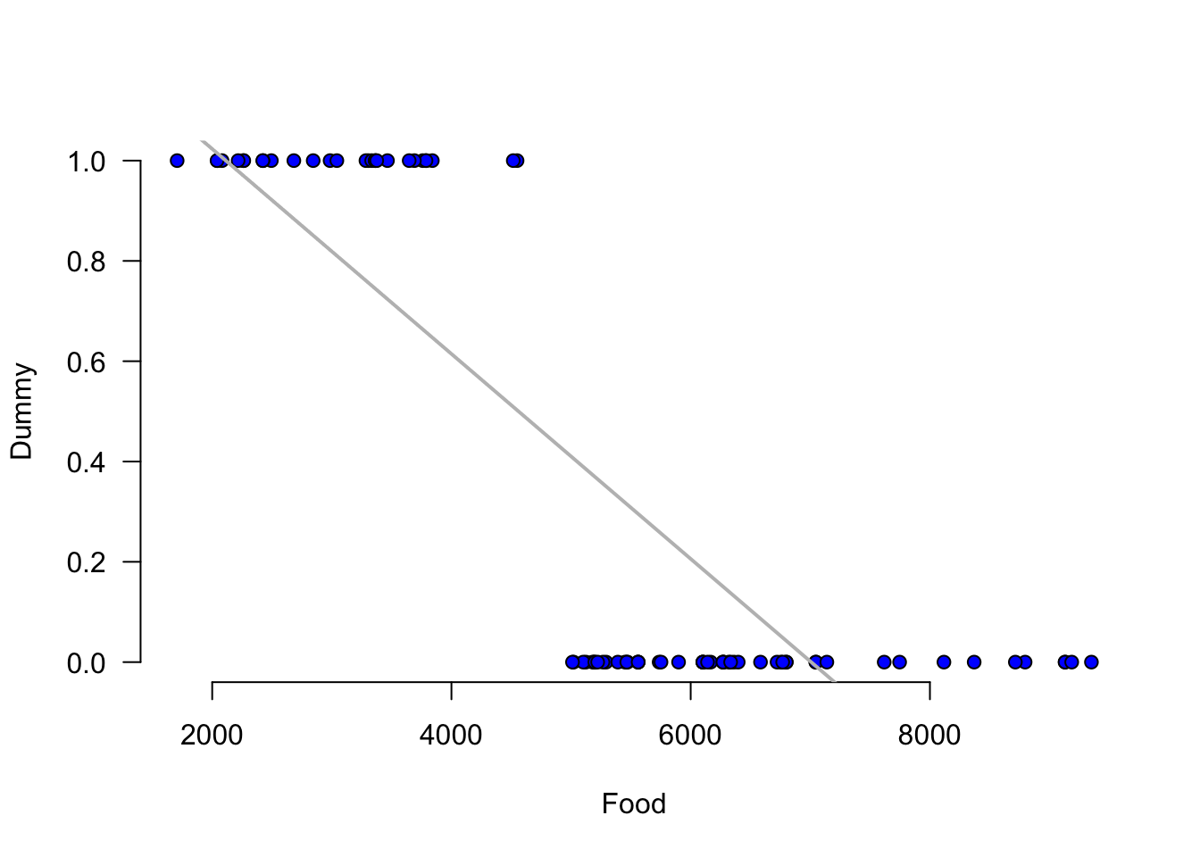
Now run a regression with Food being the independent variable and your dummy variable as the dependent variable. What is the interpretation of the intercept and slope? Hint: you might want to plot the scatter diagram and the regression line.
You will need the Population data set to answer this question. You can find this data set at https://jagelves.github.io/Data/Population.csv .
Run a regression of Population on Year. How well does the regression line fit the data?
Create a prediction for Japan’s population in 2030. What is your prediction?
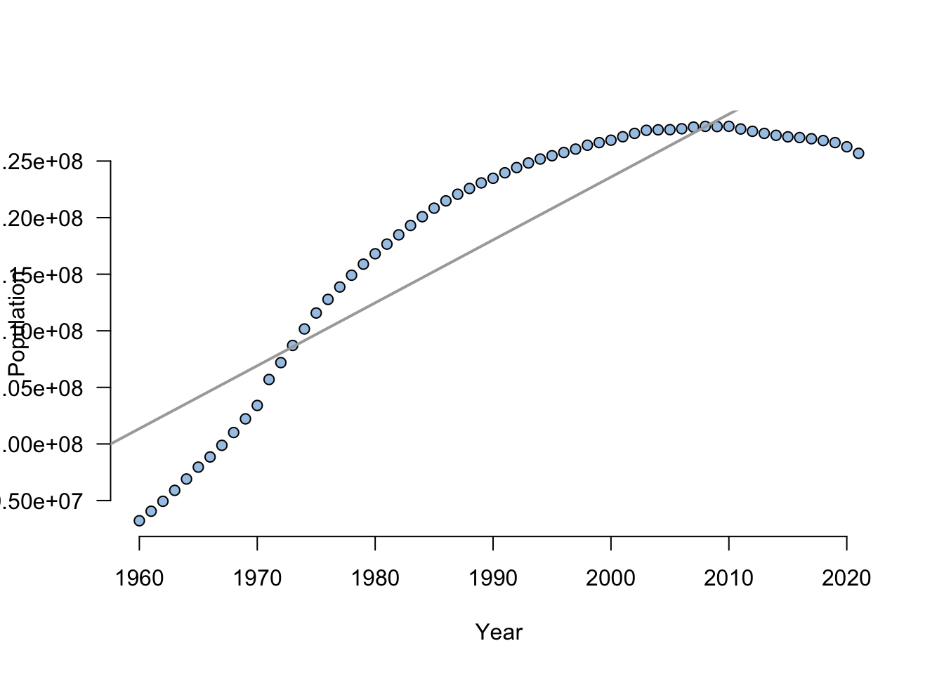
Create a scatter diagram and include the regression line. How confident are you of your prediction after looking at the diagram?
Start by generating the deviations from the mean for each variable. For x the deviations are:
x<-c(20,21,15,18,25)
(devx<-x-mean(x))[1] 0.2 1.2 -4.8 -1.8 5.2Next, find the deviations for y:
y<-c(17,19,12,13,22)
(devy<-y-mean(y))
[1] 0.4 2.4 -4.6 -3.6 5.4For the slope we need to find the deviation squared of the x’s. This can easily be done in R:
(devx2<-devx^2)[1] 0.04 1.44 23.04 3.24 27.04The slope is calculated by \(\frac{\sum_{i=i}^{n} (x_{i}-\bar{x})(y_{i}-\bar{y})}{\sum_{i=i}^{n} (x_{i}-\bar{x})^2}\). In R we can just find the ratio between the summations of (devx)(devy) and devx2.
(slope<-sum(devx*devy)/sum(devx2))[1] 1.087591The intercept is given by \(\bar{y}-\beta(\bar{x})\). In R we find that the intercept is equal to:
(intercept<-mean(y)-slope*mean(x))[1] -4.934307Our results can be easily verified by using the lm() and coef() functions in R.
fitEx1<-lm(y~x)
coef(fitEx1)
(Intercept) x
-4.934307 1.087591 Let’s start by calculating the SST. This is just \(\sum{(y_{i}-\bar{y})^2}\).
(SST<-sum((y-mean(y))^2))[1] 69.2Next, we can calculate SSR. This is calculated by the following formula \(\sum{(\hat{y_{i}}-\bar{y})^2}\). To obtain the predicted values in R, we can use the output of the lm() function. Recall our fitEx1 object created in Exercise 1. It has fitted.values included:
(SSR<-sum((fitEx1$fitted.values-mean(y))^2))[1] 64.82044The ratio of SSR to SST is the \(R^2\):
(R2<-SSR/SST)[1] 0.9367115Finally, let’s calculate SSE \(\sum{(y_{i}-\hat{y_{i}})^2}\):
(SSE<-sum((y-fitEx1$fitted.values)^2))[1] 4.379562With the SSE we can calculate the Standard Error estimate:
sqrt(SSE/3)[1] 1.208244We can confirm these results using the summary() function.
summary(fitEx1)
Call:
lm(formula = y ~ x)

Residuals:
      1       2       3       4       5
 0.1825  1.0949  0.6204 -1.6423 -0.2555

Coefficients:
            Estimate Std. Error t value Pr(>|t|)
(Intercept)  -4.9343     3.2766  -1.506  0.22916
x             1.0876     0.1632   6.663  0.00689 **
---
Signif. codes:  0 '***' 0.001 '**' 0.01 '*' 0.05 '.' 0.1 ' ' 1

Residual standard error: 1.208 on 3 degrees of freedom
Multiple R-squared:  0.9367,    Adjusted R-squared:  0.9156
F-statistic: 44.4 on 1 and 3 DF, p-value: 0.00689In R we can obtain a prediction by using the predict() function. This function requires a data frame as an input for new data.
predict(fitEx1, newdata = data.frame(x=c(32))) 1
29.86861 Start by loading the data in R:
Education<-read.csv("https://jagelves.github.io/Data/Education.csv")Next, let’s use the lm() function to estimate the regression line and obtain the coefficients:
fitEducation<-lm(Salary~Education, data = Education)
coefficients(fitEducation)
(Intercept) Education
17.258190 5.301149 Let’s get the \(R^2\) and the Standard Error estimate by using the summary() function and fitEx1 object.
summary(fitEducation)
Call:
lm(formula = Salary ~ Education, data = Education)

Residuals:
    Min      1Q  Median      3Q     Max
-62.177  -9.548   1.988  15.330  45.444

Coefficients:
            Estimate Std. Error t value Pr(>|t|)
(Intercept)  17.2582     4.0768   4.233  5.2e-05 ***
Education     5.3011     0.3751  14.134  < 2e-16 ***
---
Signif. codes:  0 '***' 0.001 '**' 0.01 '*' 0.05 '.' 0.1 ' ' 1

Residual standard error: 20.98 on 98 degrees of freedom
Multiple R-squared:  0.6709,    Adjusted R-squared:  0.6675
F-statistic: 199.8 on 1 and 98 DF,  p-value: < 2.2e-16
Lastly, let’s use the regression line to predict the salary for someone who has \(16\) years of education.
predict(fitEducation, newdata = data.frame(Education=c(16))) 1
102.0766 Start by loading the data into R and removing all NA’s:
Spend<-read.csv("https://jagelves.github.io/Data/FoodSpend.csv")
Spend<-na.omit(Spend)
To create a dummy variable for OwnHome we can use the ifelse() function:
Spend$dummyOH<-ifelse(Spend$OwnHome=="Yes",1,0)The average of the dummy variable is given by:
mean(Spend$dummyOH)[1] 0.3625To run the regression use the lm() function:
lm(Food~dummyOH,data=Spend)
Call:
lm(formula = Food ~ dummyOH, data = Spend)

Coefficients:
(Intercept)      dummyOH
6473 -3418 Run the lm() function once again:
fitFood<-lm(dummyOH~Food,data=Spend)
coefficients(fitFood)
(Intercept) Food
1.4320766616 -0.0002043632 For the scatter plot use the following code:
plot(y=Spend$dummyOH,x=Spend$Food,
     main="", axes=F, pch=21, bg="blue",
     xlab="Food",ylab="Dummy")
axis(side=1, labels=TRUE, font=1,las=1)
axis(side=2, labels=TRUE, font=1,las=1)
abline(fitFood,
       col="gray",lwd=2)
Let’s load the data from the web:
Population<-read.csv("https://jagelves.github.io/Data/Population.csv")Now let’s filter the data so that we can focus on the population for Japan.
library(dplyr)
Attaching package: 'dplyr'The following objects are masked from 'package:stats':
filter, lagThe following objects are masked from 'package:base':
intersect, setdiff, setequal, unionJapan<-filter(Population,Country.Name=="Japan")Next, we can run the regression of Population against the Year. Let’s also run the summary() function to obtain the fit and the coefficients.
fit<-lm(Population~Year,data=Japan)
summary(fit)
Call:
lm(formula = Population ~ Year, data = Japan)

Residuals:
     Min       1Q   Median       3Q      Max
-9583497 -4625571  1214644  4376784  5706004

Coefficients:
              Estimate Std. Error t value Pr(>|t|)
(Intercept) -988297581   68811582  -14.36   <2e-16 ***
Year            555944      34569   16.08   <2e-16 ***
---
Signif. codes:  0 '***' 0.001 '**' 0.01 '*' 0.05 '.' 0.1 ' ' 1

Residual standard error: 4871000 on 60 degrees of freedom
Multiple R-squared:  0.8117,    Adjusted R-squared:  0.8086
F-statistic: 258.6 on 1 and 60 DF, p-value: < 2.2e-16Let’s use the predict() function:
predict(fit,newdata=data.frame(Year=c(2030))) 1
140268585 Use the plot() and abline() functions to create the figure.
plot(y=Japan$Population,x=Japan$Year, main="",
     axes=F,pch=21, bg="#A7C7E7",
     xlab="Year",
     ylab="Population")
axis(side=1, labels=TRUE, font=1,las=1)
axis(side=2, labels=TRUE, font=1,las=1)
abline(fit,
       col="darkgray",lwd=2)