In this module, we will be learning the tools that will allow us to analyze Time Series data. Before any forecasts are estimated, we should carefully inspect the data, address any mistakes that might be present, and take note of any general patterns. Following this procedure will ensure that the data is ready for analysis.
We will first learn how to transform and manipulate our data using the dplyr package and the handy “piping” operator. We will also familiarize ourselves with the lubridate package, which helps us parse dates. Next, we will use the tsibble data structure to organize time series data. Finally, we plot the times series to identify trends, seasonality, or cyclical behavior using the ggplot2, and fpp3 packages. This last package includes the fable package used to model time series data.
4.1 Chilango’s Kitchen Wants You to Forecast Avocado Prices
Chilango’s Kitchen specializes in tacos and burritos made to order in front of the customer. Guacamole is the perfect pairing to their delicious food and one of the restaurant’s best sellers. Their guac uses just six ingredients: avocados, lime juice, cilantro, red onion, jalapeño, and kosher salt. Because of its popularity, each restaurant goes through approximately five cases of avocados daily, amounting to more than \(44,000\) pounds annually. Chilango’s Kitchen wants you to provide insights on the price of avocados in California.
4.2 The Avocado Data Set
The Hass Avocado Board provides the data set and contains weekly retail scan data of U.S. retail volume (units) and price. Retail scan data comes directly from retailers’ cash registers based on actual retail sales of Hass avocados. The data reflects an expanded, multi-outlet reporting aggregating the following channels: grocery, mass, club, drug, dollar, and military. The Average Price (of avocados) in the table reflects a per unit (per avocado) cost, even when multiple units (avocados) are sold in bags. Other avocados (e.g. greenskins) are not included in this data. You can find the data here.
Note: In general the data is recorded weekly. However, there is an entry on 01/01/2018, that is right after 12/31/2017. This is a single observation that is not weekly. There are also missing dates from 12/02/2018-12/31/2018.
4.3 Loading tidyverse and Inspecting the Data.
tidyverse is a collection of packages in R that allow us to manipulate, explore and visualize data. There are a couple of packages within tidyverse (dplyr and tidyr) that we will be using to transform our data and get it ready for analysis. dplyr will allow us to do most of our data manipulation: creating new variables, renaming variables, filtering values, sorting, grouping, and summarizing, among others. tidyr will allow us to pivot data sets, unite or separate columns, and deal with missing values. Although it is always possible to complete these tasks using base R, tidyverse allows us to efficiently perform these operations using data manipulation verbs that are very intuitive. Below we load the library.
library(tidyverse)
── Attaching core tidyverse packages ──────────────────────── tidyverse 2.0.0 ──
✔ dplyr     1.1.4     ✔ readr     2.1.5
✔ forcats   1.0.0     ✔ stringr   1.5.1
✔ ggplot2   3.5.1     ✔ tibble    3.2.1
✔ lubridate 1.9.3     ✔ tidyr     1.3.1
✔ purrr     1.0.2
── Conflicts ────────────────────────────────────────── tidyverse_conflicts() ──
✖ dplyr::filter() masks stats::filter()
✖ dplyr::lag()    masks stats::lag()
ℹ Use the conflicted package (<http://conflicted.r-lib.org/>) to force all conflicts to become errors
As you can see, several packages were attached (loaded) when we write library(tidyverse). As mentioned, both tidyr and dplyr are part of this overall package. Now that the package is loaded we can import our data by using the read_csv() function from the readr package.
Rows: 33045 Columns: 13
── Column specification ────────────────────────────────────────────────────────
Delimiter: ","
chr  (3): date, type, geography
dbl (10): average_price, total_volume, 4046, 4225, 4770, total_bags, small_b...

ℹ Use `spec()` to retrieve the full column specification for this data.
ℹ Specify the column types or set `show_col_types = FALSE` to quiet this message.
The code above imports the data as a tibble (a data structure similar to a data frame) and saves it in an object named avocado. The output informs us that three variables are classified as a character, while the rest are double. You can preview the data with either the spec() or glimpse() commands.
You will notice that the date variable is of type character. We can use the lubridate package to coerce this variable to a date. Specifically, since the date variable is formatted as month/day/year we will use the mdy() function. You can learn more about this package in Wickham (2017) Chapter 18.
library(lubridate)avocado$date<-mdy(avocado$date)
4.4 Piping and dplyr
dplyr is commonly used with “piping”. Generally speaking, “piping” allows us to chain functions. “Piping” (%>% or |>) passes the object on the left of the pipe as the first argument in the function to the right of the pipe. We can illustrate this using the select() and arrange() functions.
# A tibble: 5 × 2
  average_price geography
          <dbl> <chr>
1          3.25 San Francisco
2          3.17 Tampa
3          3.12 San Francisco
4          3.05 Miami/Ft. Lauderdale
5          3.04 Raleigh/Greensboro
There is a lot to explain in this line of code. Let’s start with the functions used. The select() and arrange() functions are part of the dplyr package. As the name indicates, the select() function selects variables from a tibble or data frame. The arrange() function sorts the data in ascending order, and the desc() function is nested inside to sort in descending order.
Let’s focus on the entire code by reading it from left to right. avocado is the tibble that contains all of the data. Since it is to the left of the pipe (%>%), it passes as the first argument of the select() function. That is why you don’t see avocado as the first argument listed in the select() function. The new data frame (i.e., the one with only the geography and the average price) then passes as the first argument of the arrange() function that follows the second pipe. The data frame is sorted in descending order so that the highest average avocado price is displayed first. Finally, the head() function is used to retrieve the top five entries.
As noted in sec-Avocado, there is an additional date in the data set that is between weeks (2018-01-01). We can remove this observation by using the filter() function.
You should notice that whereas the select() function chooses particular variables (i.e., columns), the filter() function chooses rows of the tibble that meet the conditions listed. Note also that the filtered data set is assigned (->) to avocado overwriting the older object.
The examples above highlight the use of dplyr functions to transform your data. There are plenty of other functions, but learning these are outside the scope of this book. To find out more, I recommend reading Wickham (2017) Chapter 4. Let’s use the filter() and select() functions once more to retrieve California’s average price of organic avocados for 2015-2018.
When exploring time series data, it is important to standardize the time interval between observations. The code below calculates the number of days between observations.
The pull() function vectorizes the date variable, making it possible to apply the diff() function. The result confirms that all observations are seven days apart and that no missing observations or duplicates exist.
4.5 Visualizing The Data
To visualize the data, we will be using ggplot2. One of the main functions in ggplot2 is the aes() function. This function sets the plotting canvas and determines the mapping of variables. The geom_line() function specifies the type of plot and is added to the canvas with the plus sign +. In time series, we will use the line plot regularly. Labels for the graph are easily set with the labs() function and there are plenty of themes available to customize your visualization. Below, the theme_classic() is displayed. To learn more about the ggplot package, you can refer to Wickham (2017) Chapter 2. Below is the code to create a line plot of California’s average avocado price.
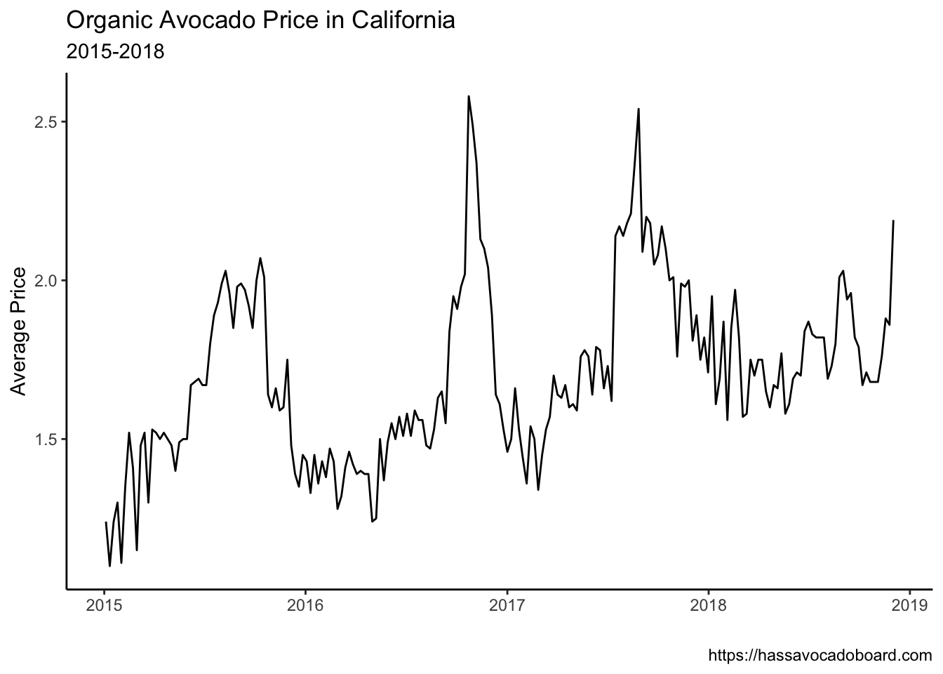
ggplot(data=cali) +geom_line(mapping=aes(x=date,y=average_price),color="black") +theme_classic() +labs(x="",y="Average Price", title="Organic Avocado Price in California",subtitle="2015-2018",caption="https://hassavocadoboard.com")
The average price of avocados in California increased during the period considered. It reached a maximum of about \(2.60\) in \(2017\) and a minimum of \(1.10\) in \(2015\). There is also a seasonal pattern with low prices at the beginning of the year and peaks mid-year. In upcoming chapters, we will extrapolate these patterns and use them to forecast time series.
4.6 tsibbles
When analyzing time series, time plays a central role. Consequently, we will use a data structure to handle a time series called a tsibble (time series tibble). tsibbles are defined by a time index (i.e., the date) that has a standard interval (i.e., days, weeks, months, and years) and keys (i.e., dimensions that do not vary with time). In the avocado data set, we are mainly interested in the average price of the avocados. You will note that the prices are classified by location (geography) and type (organic and conventional). You can learn more about tsibbles here.
tsibbles, as well a variety of packages that help us analyze time series, are part of the fpp3 package. Below we load the package, and coerce our avocado tibble to a tsibble.
In the code above, the as_tsibble() function was called with the parameter regular set at true, indicating that the date has no gaps and occurs every week (the greatest common divisor of the index column). Additionally, the type of avocado and the geography do not vary with time and are classified as a key. The function filter_index() is called as it allows us to determine the window for analysis. As noted in sec-Avocado, there are some missing dates in December 2018. We limit the analysis for now to 2015-2018.
Recall, that we are interested in the average price of avocados for California. We can specify the tsibble for analysis, by using dplyr.
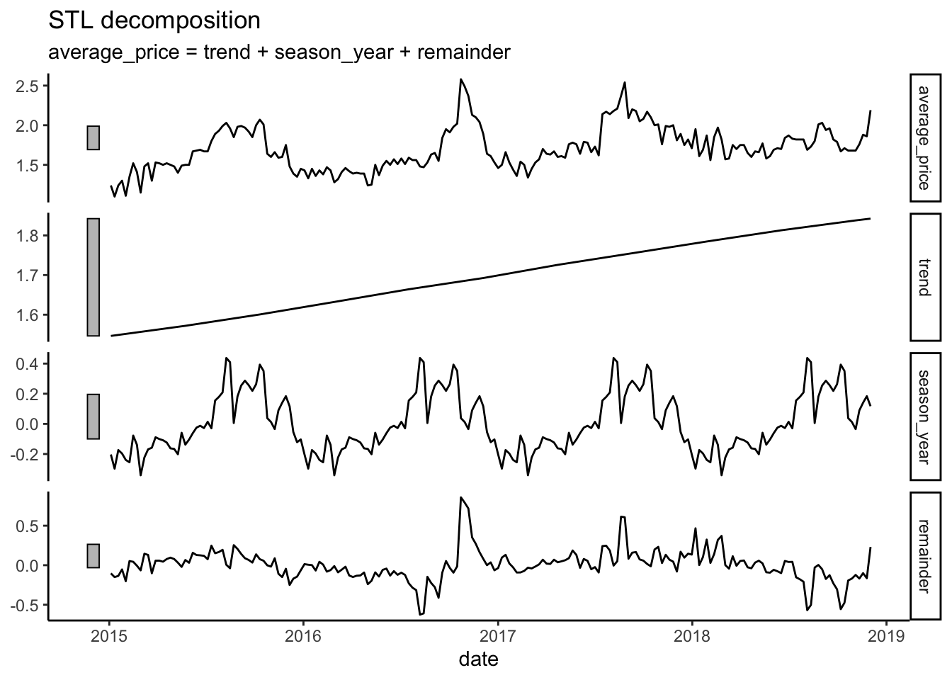
As highlighted in sec-Visual, the average price of avocados in California has a trend and a seasonal pattern. There are methods available to tease these components and make them more apparent. STL (Season Trend decomposition using LOESS) decomposes the series into a trend, seasonality, and an error (unexplained) component. It is easy to run this method in R using the fable package.
In practice, the decomposition is constructed in several steps. First, a moving average of the series is calculated to track the trend. The trend is then subtracted from the series to obtain a de-trended series. The seasonal component is calculated by averaging the values based on the window provided (52 weeks or yearly) for the de-trended series. The error is the remaining series fluctuation that is not explained by the trend or the seasonal component (\(Series-Trend-Seasonal=Error\)). In the end, each component can be graphed and displayed, as illustrated below.
fable allows us to construct this model easily by using the model() function. This function will allow us to estimate a variety of time series models, so we will be using it regularly. The particular model we are running is STL, hence the use of the STL() function within the model() function. We define the model by specifying the dependent variable (i.e., average_price) followed by a tilde (~) and the components. As you can see, the window argument in the trend() function is set to a relatively large value. By doing this the moving average reflects the general direction of the series and avoids the small fluctuations of the data. The season() function specifies \(51\) weeks to capture the yearly seasonality. Finally, the robust parameter is set to true to make the fitting process less sensitive to outliers or influential data points. Experiment by changing the window parameter to see how the decomposition changes. You can learn more about decomposition and these functions in Chapter 3 of Hyndman (2021).
As shown above, the trend is increasing, and the seasonal component confirms low levels at the beginning of the year and high levels in the summer. These are two general patterns that determine the price of avocados in California and provide valuable insight to share with Chilango’s Kitchen.
4.8 Readings
Readings get you familiar with the techniques used in time series analysis. Hyndman (2021) is the main reading here. It provides a good introduction to forecasting, plotting time series and decomposition. The book makes use of fable to conduct STL decomposition and tsibbles to capture the data. Most of time series analysis is made easier in R by using tidyverse. Wickham (2017) provides an excellent introduction to some of the packages included in tidyverse such as dplyr, ggplot, and lubridate.
Hyndman (2021) Chapter 1 (Getting Started), and Chapter 2 (Time Series Graphics), and Chapter 3 (Time Series Decomposition).
Wickham (2017) Chapter 2 (Data Visualization), Chapter 4 (Data Transformation), and Chapter 18 (Dates and Times).
In this module you have been introduced to data wrangling, plotting, tsibbles and time series decomposition. You have learned how to:
Manipulate dates with lubridate.
Select and filter variables using dplyr.
Plot time series using ggplot.
Apply tsibbles in time series analysis.
Decompose a series using the model() and STL() functions in fable.
4.10 Exercises
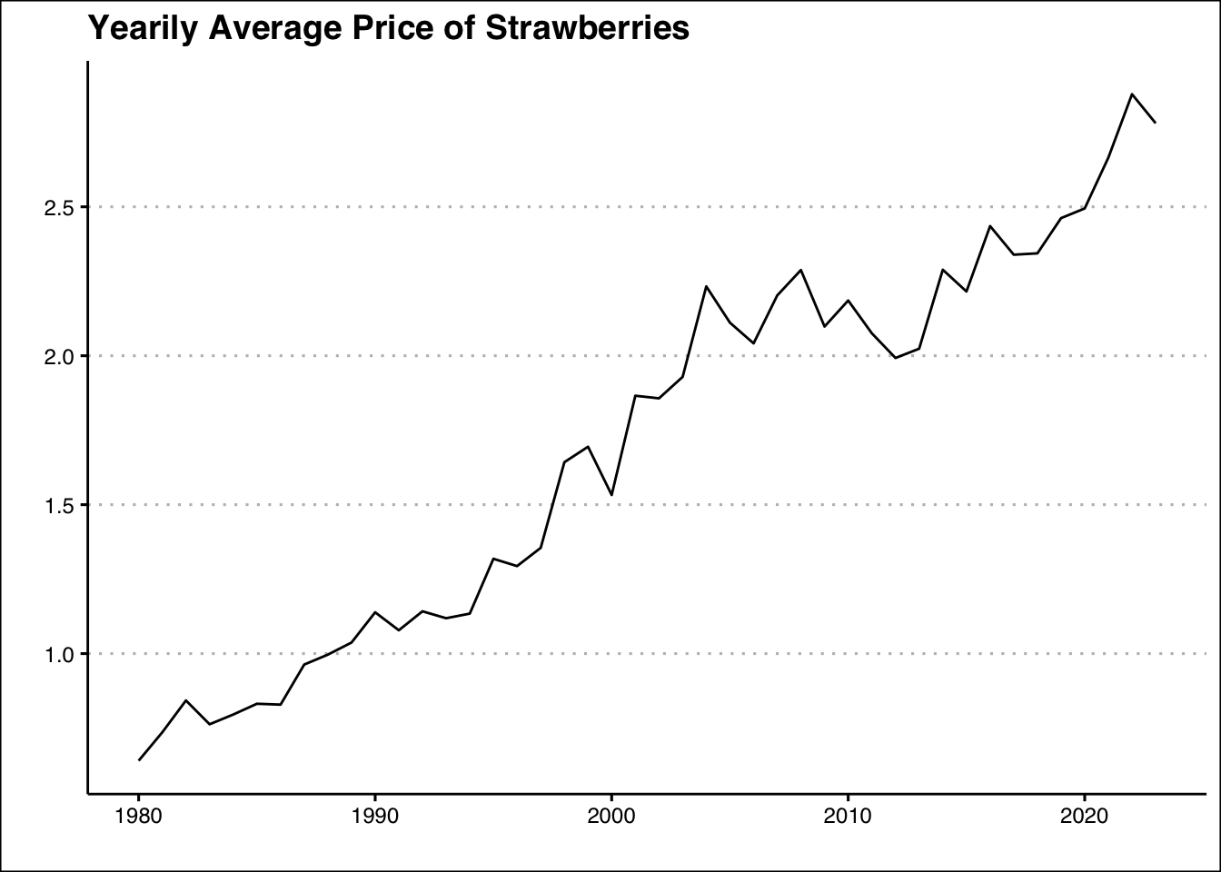
Import the following data as a tsibble with yearly data: https://jagelves.github.io/Data/StrawberryPrice.csv. Graph the time series using ggplot2 and conduct time series decomposition using the fpp3 package.
Suggested Answer
Below is code to load the libraries, and import the data:
The first mutate coerces the DATE variable to a date and extracts the year. The next mutate coerces the Price variable to a double. Lastly, the data is grouped by years and collapsed into an average. To graph we use the autoplot() command:
library(ggthemes)SB_ts %>%autoplot(.vars=APrice) +theme_clean() +labs(title="Yearily Average Price of Strawberries",y="",x="")
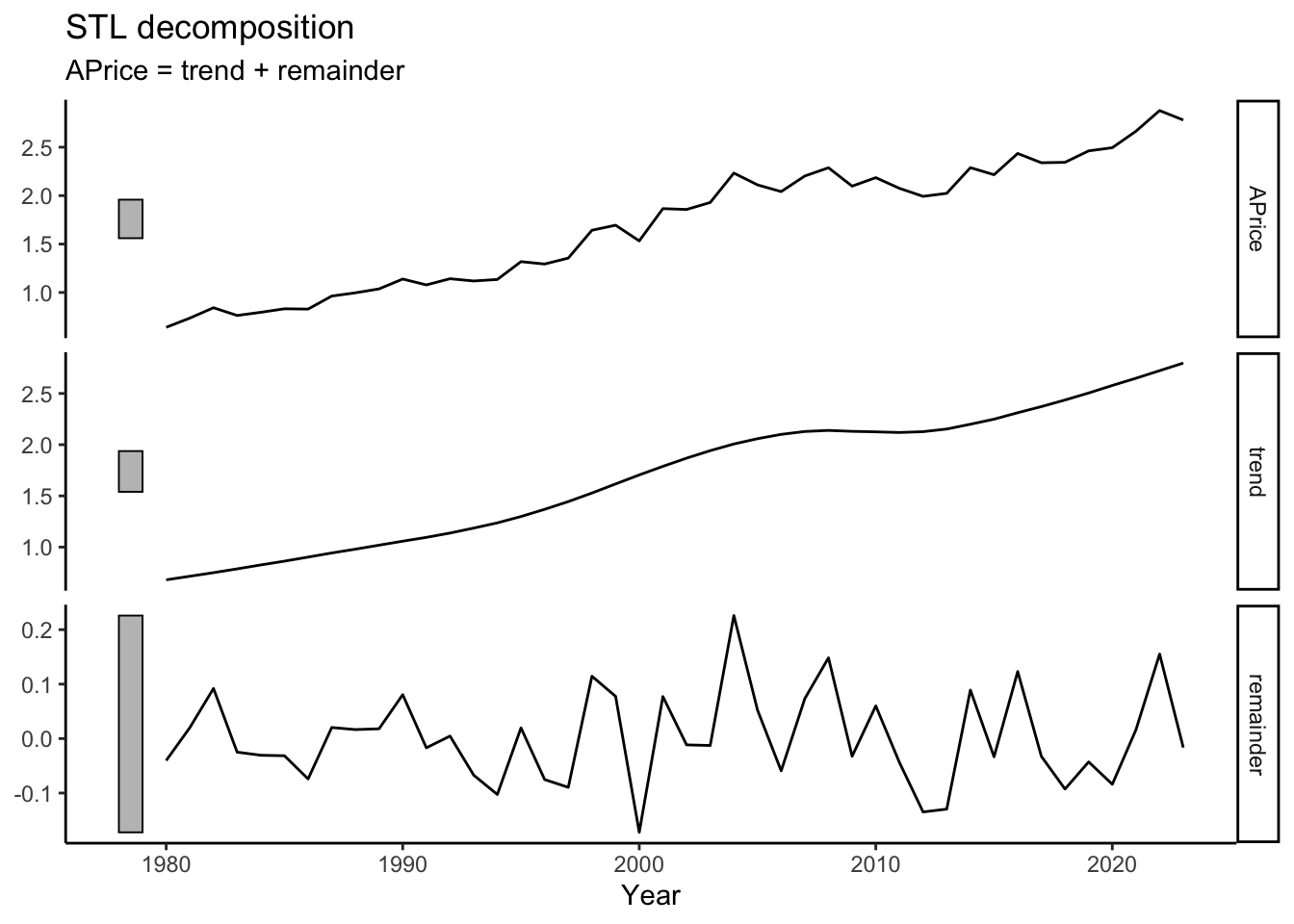
The decomposition is achieve by using the model() function:
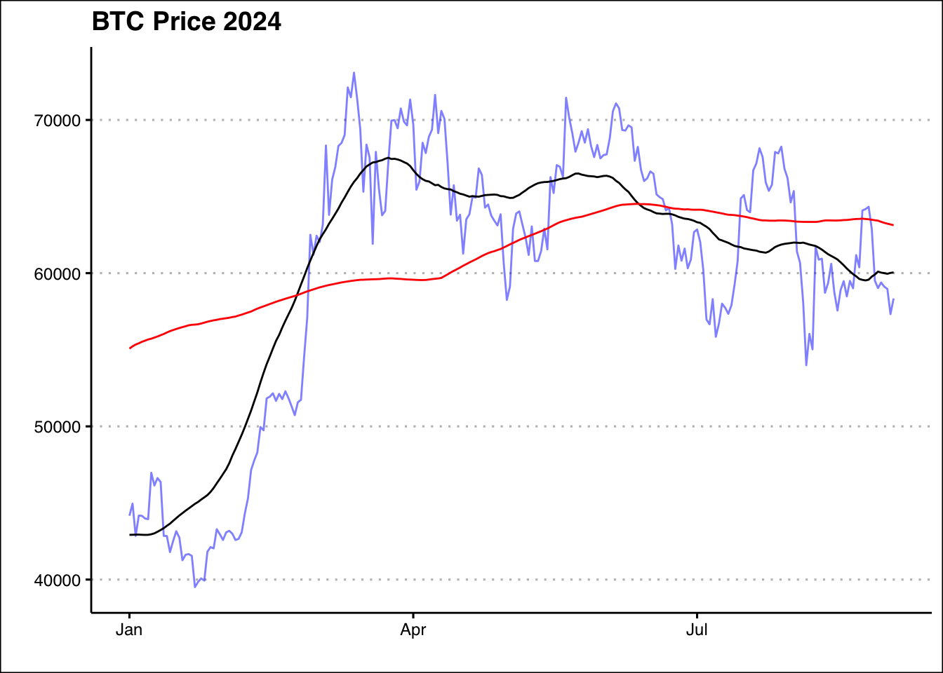
Use the dataset found below: https://jagelves.github.io/Data/BTC_USD.csv This dataset has daily Bitcoin prices for the past few years but you should focus only on 2024. Your task is to calculate two types of moving averages using the Adj Close variable, the 50-day and 200-day moving averages. After calculating these averages, you will graph the data and identify the number of times a Golden Cross and a Death Cross have occurred. A Golden Cross is a bullish signal, indicating that a stock’s price might continue to rise. It occurs when a shorter-term moving average (like the 50-day moving average) crosses above a longer-term moving average (like the 200-day moving average). A Death Cross is the opposite, representing a bearish signal and continuation to the downside. It happens when a shorter-term moving average (50-day) crosses below a longer-term moving average (200-day). How many times did these indicators guide investors correctly?
Suggested Answer
Start by importing the data and defining a tsibble:
The graph shows a golden cross at the beginning of March and a death cross mid June. The golden cross was followed by an increase in the price of BTC, and the death cross was followed by a decline in the price of BTC.
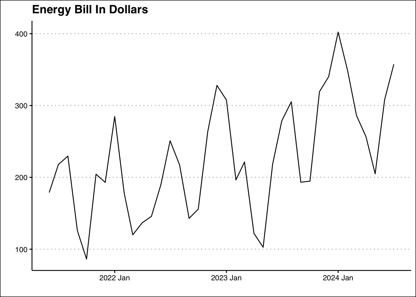
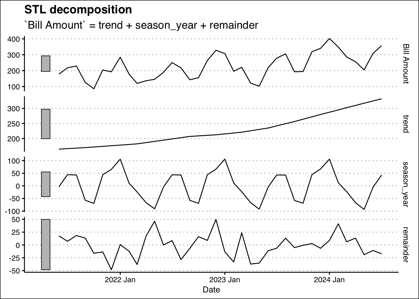
The data file: https://jagelves.github.io/Data/ElectricityBill.csv contains energy consumption from a typical U.S. household. Import the data, graph the Bill Amount variable and perform STL decomposition. Is there a clear seasonal pattern?
Suggested Answer
To import the data and create a tsibble use the following code:
The graph above shows a clear seasonal pattern. The energy bill is at its highest in the month of January, and lowest in the month of May. In general, winter and summer have higher bills than fall and spring.