3 Simulation in R

In this module we will build our first business simulation model using R. We will start by identifying and defining the parts of the model as this provides the basic structure. We will then iterate our model several times so that we can obtain the distribution of expected outcomes. Finally, we will modify some of the model’s inputs, so that we can check the robustness of our results.

3.1 Roll With It Sushi Needs Your Help

Renowned for serving the freshest sushi in the city, Roll With It Sushi is hosting a yellow-tail festival. Every morning, the Sous-Chef purchases fish at the market and any unsold fish at the end of the day gets discarded.

The restaurant has contacted you because they are still determining how many people will attend the event and worry about how this will impact their business financially. To ensure they have enough sushi and budget appropriately, they want you to recommend the amount of fish needed. Based on past events, they expect at least 20 people to attend and have the capacity to seat up to 50 guests. They anticipate the most likely attendance to be around 30 people, and without your guidance they feel like this is the best guide in determining the fish needed.

Roll With It Sushi can purchase any quantity of yellow-tail from the fresh market at 9 dollars for 16 ounces (divisible). Each guest at the festival is entitled to 5 ounces of fish. If the sushi runs out, some customers will not be happy. However, the restaurant has promised to refund their entry fee. Additionally, they have promised to serve their famous Miso soup to every attendee. The cost of making a batch for up to 50 guests is 300 dollars.

Given that the festival charges 20 dollars per entry, how much yellow-tail would you recommend the restaurant to purchase to maximize expected profits?

3.2 Model Framework

The restaurant provides you with a lot of information which might be overwhelming at first glance. To make the task less daunting, we should organize/classify the information so that we can create a model. For many business problems, the data can be classified into the following parts:

The inputs have given fixed values and provide the model’s basic structure. These are values that are most likely to be given and determined.
The decision variables are values the decision maker controls. We are usually interested in finding the optimal level of this variable.
The calculated values transform inputs and decision variables to other values that help describe our model. These make the model more informative and often are required to derive outputs.
The random variables are the primary source of uncertainty in the model. They are often modeled by sampling probability distributions.
The outputs are the ultimate values of interest; the inputs, decision variables, random variables, or calculated values determine them.

Below, you can see how we can classify and input the information in R.

library(extraDistr)
Order_Oz<-160 # Decision Variable

Price_Fish_Oz<-9/16 # Input
Price_Miso<-300 # Input
Entry_Fee<-20 # Input
Fish_Entitled_Oz<-5 #Input

set.seed(20)
Attendance<-round(rtriang(1,20,50,30),0) # Random Variable

Demand<-Attendance*Fish_Entitled_Oz # Calculated 
Available<-Order_Oz # Calculated
Consumption<-min(Demand,Available) #Calculated
Revenue<-Consumption/Fish_Entitled_Oz*Entry_Fee# Calculated
Cost<-Order_Oz*Price_Fish_Oz+Price_Miso #Calculated
Profit<-Revenue-Cost # Outcome

In the model above, you can see how the inputs have fixed values. These values were given to us by the restaurant and the restaurant has little or no control over them (the market price of the fish, the cost of making Miso soup, etc.). The random variable, captures the source of uncertainty (i.e., how many people attend the event). As you can see we have used here the rtriang() function from the extraDistr package to generate the attendance. We have chosen the triangle distribution since the restaurant has provided us with a lower limit (20), an upper limit (50), and a most likely case for attendance (30). Note also the use of the set.seed() function. This allows you to replicate the random numbers generated.

The calculated variables combine inputs, the decision variable, and the random variable to provide insight on how much is fish is expected to be both consumed and available. They also help us determine the profit (output), which is our main guide in knowing whether the decision of ordering $x$ ounces of fish is the “best”.

3.3 The News Vendor Problem

Note how the decision variable (Order_Oz) affects directly our outcome (Profit). We can see that it decreases the restaurant’s profit through costs, but also affects revenue through the amount of fish available. This is the heart of the problem. We don’t know how many people will attend, so if the restaurant orders too much fish their profits will go down because their costs are large. However, if they order too little then they will have to issue refunds, which decrease their revenue.

As you observe the Profit formula in the code above, you’ll notice the use of the min() function. This function returns the minimum of the Attendance and Consumption. The intuition here is that the restaurant can only collect entry fees for people who consumed sushi when the attendance is greater than the amount of sushi available. Likewise, their revenue will be capped at the total amount of people who attended, even if they ordered plenty of fish.

The problem illustrated above is called the news vendor problem. The news vendor problem is a classic decision-making problem in operations research and economics that involves deciding how much of a product to order (and sometimes at what price to sell it). The problem is called the “news vendor” problem because it was originally used to model the decision-making process of a newspaper vendor trying to decide how many copies of a newspaper to order and at what price to sell them.

3.4 Law of Large Numbers

Before we answer the question of how much fish to order, we must realize a couple of flaws of the model we have created. Mainly, we have run the simulation once and it is unlikely (although possible) that the attendance will be exactly the single value simulated by the rtriang() function ($44$). Instead, we want to provide the restaurant with a set of eventualities. Worst case scenarios (low attendance), best case scenarios (high attendance), and most likely outcome for their decision. This is only possible if we generate several attendance numbers, and see how the profit (output) behaves.

An additional problem is that if we tell the restaurant that the expected profit of ordering $x$ amount of fish is $y$, we want to make sure that the average is not biased. Recall that as the sample size of a study increases, the average of the sample will converge towards the true population mean. In other words, as the number of simulations in our model increases, the estimate of the expected profit becomes more accurate. This is known as the Law of Large Numbers.

The code below repeats the simulation several times, allowing for different attendance scenarios to arise. Although, there is not a set number of times one should run a simulation to get a good estimate of the mean (or distribution), computers are powerful enough to run thousands if not millions of simulations. Below we run the simulation 10,000 times for illustration purposes.

n<-10000
V_Order_Oz<-rep(Order_Oz,n)
V_Price_Fish_Oz<-rep(Price_Fish_Oz,n)
V_Price_Miso<-rep(Price_Miso,n)
V_Entry_Fee<-rep(Entry_Fee,n)
V_Fish_Entitled_Oz<-rep(Fish_Entitled_Oz,n)

set.seed(12)
V_Attendance<-round(rtriang(n,20,50,30),0)
V_Demand<-V_Attendance*V_Fish_Entitled_Oz
Available<-V_Order_Oz

V_Consumption<-pmin(V_Demand,Available) 
V_Revenue<-V_Consumption/Fish_Entitled_Oz*Entry_Fee
V_Cost<-Order_Oz*Price_Fish_Oz+Price_Miso
V_Profit<-V_Revenue-V_Cost

In the code above, you will notice that operations have been vectorized to avoid the use of for loops. For example, the order (Order_Oz) has been repeated 10000 times. By doing this, the inputs can now be combined with the randomly generated attendance (V_Attendance). Finally, note as well the use of the pmin() function instead of the min() function. This allows us to apply the min() function to each element (rows) of the vectors.

From the simulation it seems like that the restaurant would make on average a profit of about $211.5$ dollars if they order $160$ ounces of fish. There are however, a couple of questions left unanswered. First, what are the other possible profits when ordering $160$ ounces? Second, is there another amount of fish that would give them a higher expected profit?

3.5 Flaw Of Averages

To answer the first question we can generate a histogram of all the results of our simulation model. We can then report this to the restaurant and make them aware of all of the possible outcomes of ordering $160$ ounces of fish. Below, we show the histogram of our model’s outcomes.

hist(V_Profit, main="Expected Profits of an Order of 160 Ounces",
     xlab="")
abline(v=mean(V_Profit), lwd=2)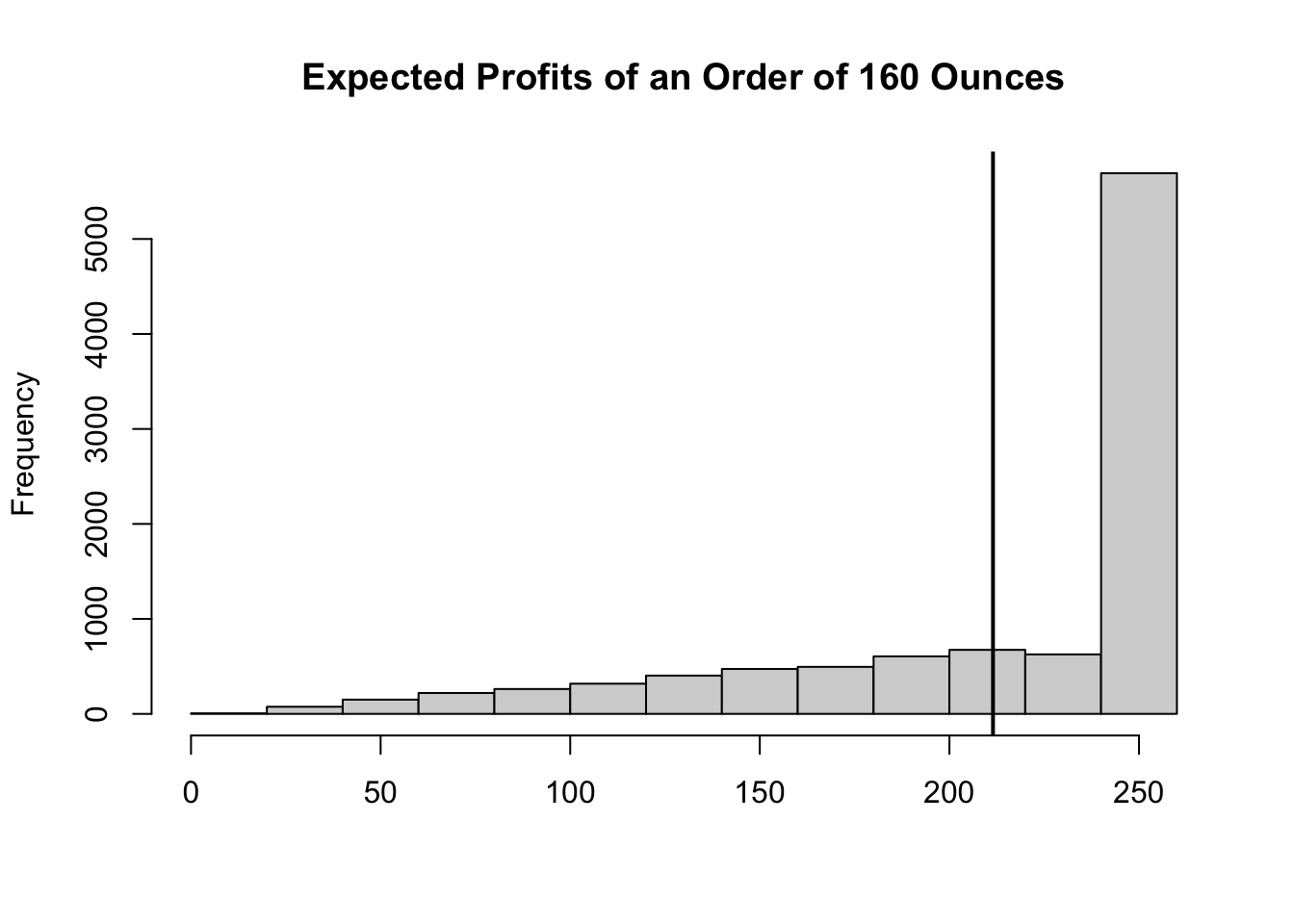

As you can see most of the outcomes are close to $250$ dollars. So a better recommendation to the restaurant would be to inform them that when ordering $160$ ounces, they will most likely get a profit of $250$ dollars. There is a small risk of them making less that $100$ dollars in profit, but that they should not expect more than $250$ dollars. The average in this case seems to be a poor predictor of what is expected as its frequency is not very large as shown in the histogram. This result is known as the flaw of averages.

The flaw of averages, also known as the “law of averages fallacy,” is the idea that the average value of a particular characteristic in a population can be used to represent the value of that characteristic for individual members of the population. This is often not the case because the average value can be misleading and does not take into account the variability and distribution of the characteristic within the population.

3.6 Optimal Order Amount

Now to answer the main question, what should be the amount ordered of fish? To answer this question we will substitute several possible order options into our model and then retrieve the one that gives us the highest expected profit. We can easily do this in R with a for loop. Below is the code:

Order_Oz=seq(160,240,10)
Price_Fish_Oz<-9/16 
Price_Miso<-300 
Entry_Fee<-20 
Fish_Entitled_Oz<-5 

Profits<-c()

for (i in Order_Oz){
n<-100000
V_Order_Oz<-rep(i,n)
V_Price_Fish_Oz<-rep(Price_Fish_Oz,n)
V_Price_Miso<-rep(Price_Miso,n)
V_Entry_Fee<-rep(Entry_Fee,n)
V_Fish_Entitled_Oz<-rep(Fish_Entitled_Oz,n)

set.seed(12)
V_Attendance<-round(rtriang(n,20,50,30),0) 
V_Demand<-V_Attendance*V_Fish_Entitled_Oz 
Available<-V_Order_Oz

V_Profit<-pmin(V_Demand,Available)/V_Fish_Entitled_Oz*V_Entry_Fee-V_Order_Oz*V_Price_Fish_Oz-V_Price_Miso
Profits<-c(Profits,mean(V_Profit))
}

(results<-data.frame(Order=Order_Oz,Profits=Profits))

  Order  Profits
1   160 212.0358
2   170 225.7342
3   180 235.1670
4   190 240.7776
5   200 243.1558
6   210 242.8690
7   220 240.4326
8   230 236.4392
9   240 231.4190

This table suggests that ordering $160$ ounces is not optimal. Once again highlighting that the average attendance is not a good estimate of how much fish we should order. Instead, we can see that $200$ ounces of fish should be ordered (this feeds $40$ people) to maximize the expected profits ($243$ dollars).

3.7 Sensitivity Analysis

What if the price of yellow-tail increases unexpectedly? What if the restaurant wishes to provide each guest with six ounces of fish instead of five? The model we have created above can accommodate these changes easily by just changing the input values. We can additionally, inform the restaurant how sensitive the results are to changes in key inputs or assumptions. This is the idea behind sensitivity analysis.

Sensitivity analysis assesses the robustness of a model or decision by evaluating the impact of changes in certain key input variables on the output of the model or decision. Sensitivity analysis helps to identify which variables are most important and how sensitive the output is to changes in those variables.

Let’s consider providing each guest with six or seven ounces of fish. How does this change our recommendation? When running our model with different amounts of fish provided, you’ll notice that when each guest gets six ounces of fish, the restaurant should order $240$ ounces yielding an expected profit of $220$ dollars. When each guest gets seven ounces of fish, the restaurant should order $270$ ounces which generates an expected profit of $198$ dollars. Perhaps providing each guest with more fish is a bad idea as profits are highly sensitive to every ounce increase.

3.8 Readings

The readings for this chapter will introduce the application of simulation models to business. Winston and Albright (2019) highlight the technical application of the models using Excel. It is recommended that you follow in R instead. Kwak and Ingall (2007) motivates the use of Monte Carlo simulation for managing project risks and uncertainties.

Winston and Albright (2019) Chapter 10.3 (Simulation and the Flaw of Averages), and 10.4 (Simulation with Built-In Excel Tools). Example 10.4 (Additional Uncertainty at Walton Bookstore) It is recommended you follow along using R instead of Excel.
Kwak and Ingall (2007)

3.9 Lessons Learned In This Chapter

Identify the parts of a simulation model.
Create a simulation model in R.
Identify the Flaw of Averages.
Find optimal values in simulation models

3.10 Exercises

Apple is preparing to launch a special edition smartphone accessory designed exclusively for its latest iPhone. This accessory is only compatible with this specific model, and the company anticipates that demand will peak during the first 12 months following the smartphone’s release. After this period, a new model of the smartphone is expected to be released, rendering the accessory obsolete. The company estimates that demand for the accessory during the twelve-month period is governed by the probability distribution in the table below.

The production involves a fixed cost of 20,000 dollars, with a variable cost of 15 dollars per unit produced. Each accessory is sold for 100 dollars. However, any unsold units after the twelve-month period will have no value, as they are not compatible with the newest iPhone.

The company is considering producing 10,000 units of the accessory. Using a simulation with 100,000 replications, calculate the expected profit and standard deviation. Additionally, determine the range within which the company can be 90% certain that the actual profit from selling the accessory during the twelve-month period will fall.

Demand (units)	Probability (%)
6,000	10%
7,000	20%
8,000	30%
9,000	25%
10,000	15%

Suggested Answer

Expected Profit: 645,000

Standard Deviation: 119,326

90% Confidence Interval: [430,000, 830,000]

Alaska Airlines is preparing for the peak holiday travel season and needs to decide how many seats to overbook on the SEA-SFO route. Overbooking is expected in the airline industry, as some passengers typically do not show up for their flights. The airline has data indicating that the number of no-show passengers on this route follows a normal distribution with a mean of 20 and a standard deviation of 5.

If the airline does not overbook enough seats, empty seats result in lost revenue, as the cost of an unused seat is estimated to be $300. However, if the airline overbooks too many seats, it may need to compensate bumped passengers with vouchers worth $600 each. Use 10,000 simulations to determine the optimal number of seats to overbook to minimize the airline’s expected cost. Try possible values from 10 to 30 in increments of 5.

Suggested Answer

Optimal Overbooking Strategy: 18 seats

Minimum Expected Cost: $1,633

The Bronco Wine Company is planning to launch a special edition of its finest wine for the upcoming holiday season. The winery faces uncertainty in both customer demand and grape yield, which affects production.

Demand is modeled by a triangular distribution with a minimum of 500, most likely 1,500, and maximum of 2,500 bottles. Production Costs are 10,000 dollar fixed plus 15 dollars per bottle. Selling Price is 100 dollars per bottle. Salvage Value is 30 per unsold bottle (up to 1,000 bottles). The maximum number of bottles that can be produced is also uncertain and follows a Beta distribution with parameters α = 2 and β = 5, scaled to a maximum capacity of 3,000 bottles. The winery is considering production levels ranging from 1,000 to 3,000 bottles in increments of 500.

Use 10,000 simulations to determine the optimal number of bottles to produce to maximize the winery’s expected profit. Create a five number summary to describe the distribution of profits at the optimal number of bottles.

Suggested Answer

Optimal Production Level: 1,500

Expected Profit: $47,663

Min: -32500, Q1: 15900, Median:46100, Q3:78020, Max:117500

You are considering an investment in the SPY (S&P 500 ETF) over a 20-year period. Your investment strategy involves making an initial investment, followed by yearly contributions.

The key parameters for your investment are as follows:
- Stock Ticker: SPY (S&P 500 ETF)
- Initial Investment: $1,000
- Average Yearly Return: 10% (0.1)
- Standard Deviation of Yearly Returns: 18% (0.18)
- Yearly Investment: $6,000
- Investment Period: 20 years
Run 10,000 simulations of your investment over 20 years. Each year, returns are normally distributed with the given average and standard deviation. Track the value of your investment at the end of each year. Calculate the following statistics for the investment value at the end of 20 years:
- Average (mean) end value
- Worst Case Scenario: Minimum
- Bear Case: 25th percentile (Q1)
- Base Case: Median (50th percentile)
- Bull Case: 75th percentile (Q3)
- Best Case Scenario: Maximum
Based on your simulation results, how much can you expect to have in your account after 20 years on average? What are the Bear, Base and Bull case predictions?

Suggested Answer

Expected End Value after 20 years: $380,000

Bear Case: $233,000

Base Case: $332,000

Bull Case: $476,000

You are tasked with simulating the price of BTC (Bitcoin) over one year using Brownian motion and plotting the result. Brownian motion is a mathematical model used to describe random motion, often applied in finance to simulate stock price movements. In particular, the returns of a stock are described by the following equation: $\text{returns} = (\mu - 0.5 \times \sigma^2) \times dt + \sigma \times \sqrt{dt} \times \epsilon$; where $\epsilon$ is a random shock drawn from a standard normal distribution, $\mu$ is the expected annual return, $\sigma^2$ is the variance of returns, and $dt = 1/365$. Assume that the starting Bitcoin price is 50,000 dollars, with an average return of 40% and standard deviation of 100%. Let the path of Bitcoin be given by: $Price=S0*cumprod(1+returns)$; where $S0$ is the initial price. Generate 1000 price paths using Brownian motion (set seed to 150). Report the mean, bear (Q1), base (Q2) and bull cases (Q3) of the final prices after 1 year.

Suggested Answer

Expected End Value 1 year (365 days): $48,293

Bear Case (Q1): $13,642

Base Case (Q2): $27,306

Bull Case (Q3): $58,680