set.seed(15)
Population<-runif(1000,100,200)11 Inference I
Statistical inference is a cornerstone of modern business decision-making. It enables companies to extract meaningful insights from data amid uncertainty and complexity. Businesses can predict customer behavior, optimize marketing strategies, and assess risks by drawing reliable conclusions from sample data. In this chapter, we explore how we can draw insights from the population using sample data.
11.1 Statistical Inference
The power of statistical inference lies in allowing us to learn about a population by studying the properties of the sample. The process relies on estimating a sample statistic, like the sample mean (i.e., the sample statistic). The sample mean gives us a good guess about the population mean (i.e., the population parameter), as long as it comes from a fair and random selection. Certain qualities or properties of the sample mean enable us to make sound inference of the population parameter. Below, we study the properties of unbiasedness, consistency, and efficiency (asymptotic normality).
11.2 Unbiasedness
Simply put, unbiasedness states that expected value of the sample means is equal to the population mean. Formally,
\[E[\bar{X}] = \mu\] To convince ourselves of this property, consider the data below as being the population.
| \(x_1\) | \(x_2\) | \(x_3\) | \(x_4\) |
|---|---|---|---|
| 3 | 12 | 18 | 30 |
In this example, we have access to the entire population, consisting of the four numbers {3, 12, 18, 30}. This allows us to calculate the population mean as:
\[\mu = \frac{3 + 12 + 18 + 30}{4} = 15.75\]
In practice, population data is rarely available, and we rely on samples to estimate population parameters. Consider taking a random sample of three elements from this population. The table below lists all possible samples of size three, along with their corresponding sample means.
| Sample | Sample Outcome | \(\bar{x}\) |
|---|---|---|
| 1 | {3,12,18} | \(\bar{x}_1=11\) |
| 2 | {3,12,30} | \(\bar{x}_2=15\) |
| 3 | {3,18,30} | \(\bar{x}_3=17\) |
| 4 | {12,18,30} | \(\bar{x}_3=20\) |
Upon examining the table, it is evident that none of the sample means (\(\bar{x}_1, \bar{x}_2, \bar{x}_3, \bar{x}_4\)) equals the population mean (\(\mu = 15.75\)). This discrepancy is known as sampling error. Formally, sampling error is defined as the difference between a sample statistic, such as the sample mean, and the corresponding population parameter:
\[ Sampling\ Error=\bar{x}-\mu\] Sampling error is not the result of mistakes or biases in the sampling process; rather, it is a natural consequence of sampling variability, as illustrated by the varying sample means in the table. Intuitively, the sampling error would be zero if the sample included the entire population, but it could be substantial with a very small sample, such as a single element. Generally, sampling error tends to decrease as the sample size increases, as larger samples provide more accurate estimates of the population parameter.
Note
To explore how the sampling error changes with the sample size press here.
A critical insight from the table emerges when we calculate the mean of the sample means. Summing the sample means and dividing by the number of samples:
\[\frac{\bar{x}_1 + \bar{x}_2 + \bar{x}_3 + \bar{x}_4}{4} = \frac{11 + 15 + 17 + 20}{4} = \frac{63}{4} = 15.75\]
Remarkably, this value is exactly equal to the population mean, \(\mu = 15.75\). This is not a coincidence but a demonstration of a fundamental unbiasedness property. In statistical terms, an estimator is unbiased if its expected value equals the true population parameter. Once more, this is expressed as: \[E[\bar{X}] = \mu\] In this context, the mean of all possible sample means represents the expected value of the sample mean, and it precisely matches the population mean. This property underscores that, despite individual sample means deviating from \(\mu\) due to sampling error, the sample mean is, on average, an accurate estimator of the population mean.
Far from being disconnected, the sample mean and population mean are strongly related through the concept of unbiasedness. While any single sample mean may differ from \(\mu\) due to sampling variability, the unbiasedness property ensures that, over all possible samples, the sample mean centers on the true population mean. This relationship is the cornerstone of statistical inference, allowing us to use sample data to make reliable inferences about unknown population parameters. In practice, when population data is unavailable, the unbiasedness of the sample mean provides confidence that our estimates are, on average, correct, bridging the gap between sample statistics and population parameters.
11.3 Consistency
The property of consistency states that as the sample size increases, the sample mean converges in probability to the population mean. As we saw in the table above, different samples yield different sampling errors, with some errors being larger than others. This variability is random and depends on the specific sample drawn. Consistency ensures that larger samples produce more accurate estimates, meaning the probability that the sample mean deviates from the population mean \(\mu\) by more than any fixed amount \(\epsilon\) approaches zero as the sample size grows.
Example: Consider the population {3, 12, 18, 30}, with a population mean \(\mu = 15.75\). To illustrate consistency, let’s compare the sampling errors for samples of size two, size three, and size four (the entire population).
Below is a table listing all possible samples of size two, along with their sample means and sampling errors:
| Sample | Sample Outcome | \(\bar{x}\) | \(\bar{x} - \mu\) |
|---|---|---|---|
| 1 | {3,12} | \(\bar{x}_1 = \frac{3+12}{2} = 7.5\) | \(-8.25\) |
| 2 | {3,18} | \(\bar{x}_2 = \frac{3+18}{2} = 10.5\) | \(-5.25\) |
| 3 | {3,30} | \(\bar{x}_3 = \frac{3+30}{2} = 16.5\) | \(0.75\) |
| 4 | {12,18} | \(\bar{x}_4 = \frac{12+18}{2} = 15\) | \(-0.75\) |
| 5 | {12,30} | \(\bar{x}_5 = \frac{12+30}{2} = 21\) | \(5.25\) |
| 6 | {18,30} | \(\bar{x}_6 = \frac{18+30}{2} = 24\) | \(8.25\) |
The sampling errors range from \(-8.25\) to \(8.25\), with an average absolute error of: \[\frac{|-8.25| + |-5.25| + |0.75| + |-0.75| + |5.25| + |8.25|}{6} = \frac{8.25 + 5.25 + 0.75 + 0.75 + 5.25 + 8.25}{6} = 4.75\]
Similarly, the average absolute error for a sample size of three is given by: \[\frac{|-4.75| + |-0.75| + |1.25| + |4.25|}{4} = \frac{4.75 + 0.75 + 1.25 + 4.25}{4} = 2.75\]
The sampling error for the population is: \[\bar{x} - \mu = 15.75 - 15.75 = 0\]
11.4 Precision
In simple terms, the precision property of the sample mean ensures that as the sample size grows, the sample mean becomes a more reliable and tightly clustered estimate of the population mean. This follows from the fact that the standard deviation of the sample means or standard error (\(\sigma_{\bar{x}} = \sigma / \sqrt{n}\)) is lower than the population standard deviation (\(\sigma\)).
Let’s consider once more the population data below:
| \(x_1\) | \(x_2\) | \(x_3\) | \(x_4\) |
|---|---|---|---|
| 3 | 12 | 18 | 30 |
The population variance is given by:
\(\sigma^2 = \frac{(3-15.75)^2 + (12-15.75)^2 + (18-15.75)^2 + (30-15.75)^2}{4} = 96.1875\)
For a sample size of \(n=3\), the variance of the sample means, adjusted for a finite population of size \(N=4\), is:
\(\frac{\sigma^2}{n} \times \frac{(N-n)}{(N-1)} = \frac{96.1875}{3} \times \frac{(4-3)}{(4-1)} = 32.0625 \times \frac{1}{3} = 10.6875\)
Notice how the sample size \(n\) inversely affects the variance of the sample mean. As the sample size increases, the variance of the sample mean decreases, leading to more precise estimates. The equation above may not be immediately intuitive, so we verify it by calculating the variance using the sample means directly. Recall the sampling distribution data for samples of size \(n=3\):
| Sample | Sample Outcome | \(\bar{x}\) | \((\bar{x}-\mu)^2\) |
|---|---|---|---|
| 1 | {3,12,18} | \(\bar{x}_1=11\) | 22.5625 |
| 2 | {3,12,30} | \(\bar{x}_2=15\) | 0.5625 |
| 3 | {3,18,30} | \(\bar{x}_3=17\) | 1.5625 |
| 4 | {12,18,30} | \(\bar{x}_4=20\) | 18.0625 |
The variance of the sample means is:
\(\text{Var}(\bar{x}) = \frac{22.5625 + 0.5625 + 1.5625 + 18.0625}{4} = 10.6875\)
As a final note, most population data we consider is sufficiently large so that we don’t have to adjust the measure of standard error. The standard error is then given by \(\sigma_{\bar{x}} = \sigma / \sqrt{n}\) and not \(\frac{\sigma} {\sqrt{n}} \times \sqrt{\frac{(N-n)}{(N-1)}}\).
In sum, the property of precision demonstrates that the variance of the sampling distribution is less than the population variance, and more importantly, as the sample size increases, the sample mean becomes an increasingly accurate estimator of the population mean.
11.5 Asymptotic Normality and the Central Limit Theorem
We have explored the desirable properties of estimators. However, to construct confidence intervals or perform hypothesis tests, we need to know (or approximate) the shape of the sampling distribution of an estimator, not just its center and spread. For small samples from non-normal (or binary) populations, this shape can be unpredictable and inconvenient.
This is where the Central Limit Theorem (CLT) emerges as one of the most profound and practical results in statistics. The CLT states that, regardless of the underlying population distribution (provided it has finite variance), the standardized sample mean becomes approximately normally distributed as the sample size (\(n\)) grows large:
\[ \frac{\bar{X} - \mu}{\sigma / \sqrt{n}} \approx N(0, 1)\]
This convergence to normality—building directly on the precision gains we have seen—enables us to use the familiar normal (or \(z\)) table for probabilistic statements, even when the original data are skewed, discrete, or non-normal. The same principle applies to the sample proportion (\(\hat{p}\)), where the sampling distribution of the sample proportion is also normally distributed for a sufficiently large (\(n\)).
\[ \frac{\hat{p} - p}{\sqrt{p(1-p)/n}} \approx N(0, 1) \]
In summary:
For the sample mean ({X}): - If the population is normal, the sampling distribution of (\(\bar{X}\)) is exactly normal (for any (\(n\))). - If the population is non-normal, the sampling distribution of (\(\bar{X}\)) is approximately normal for large (\(n\)) (typically (\(n > 30\))).
For the sample proportion (): - The underlying “population” is binary (success probability (\(p\))), so normality is only approximate.
- The approximation is good when (\(np \geq 10\)) and (\(n(1-p) \geq 10\)) (or more conservatively (\(geq 15\))); in practice, we check these using the estimated (\(\hat{p}\)).
Thus, with sufficiently large random samples satisfying the relevant conditions, both (\(\bar{X}\)) (mean (\(\mu\)), standard error (\(\sigma / \sqrt{n}\))) and (\(\hat{p}\)) (mean (\(p\)), standard error (\(\sqrt{p(1-p)/n}\))) follow approximate normal distributions, regardless of the population’s shape.
Note
To explore central limit theorem and how the sample size affects the sampling distribution press here.
11.6 Some Details on Proportions
Statistical inference can also be performed with proportions (e.g. the proportion of left handed people, proportion of people with a particular virus, etc.). We can relate this proportions to the outcome of a binomial distribution. Recall that the binomial distribution describes the number of successes \(x\) in \(n\) trials of a Bernoulli process where \(p\) is the probability of success. Here, \(x/n\) is the proportion of successes.
To estimate the population proportion use the sample proportion \(\bar p = x/n\). This estimate is unbiased (i.e., \(E(\bar p)=P\)), where \(P\) is the population proportion.
The standard error of the estimate is \(se(\bar P)= \sqrt { \frac {p(1-p)}{n}}\), where \(p\) is the sample proportion, and \(n\) is the sample size.
By the central limit theorem, the sampling distribution of \(\bar p\) is approximately normal when \(np \geq 5\) and \(n(1-p)\geq 5\).
11.7 Useful R Functions
Here are some functions that are handy when simulating data in R.
The pnorm() and punif() functions calculate probabilities for the normal and uniform distributions, respectively.
The rnorm() and runif() functions generate random numbers from a normal and uniform distribution, respectively.
The for() function creates a loop that repeats a procedure a specified amount of times.
The set.seed() function is used to create reproducible results in R when random numbers are used.
11.8 Exercises
The following exercises will help you test your knowledge on the Inference. In particular, the exercises work on:
The Central Limit Theorem.
Sampling Distribution for means.
Sampling Distribution for proportions.
Answers are provided below. Try not to peak until you have a formulated your own answer and double checked your work for any mistakes.
Exercise 1
In this exercise we will be simulating the central limit theorem. You will need R to complete this problem.
- Create a random sample of 1000 data points and store it in an object called Population. Use the uniform distribution with min of 100 and max of 200 to generate the sample. Calculate the mean and standard deviation of the random sample and call PopMean and PopSD, respectively.
Answer
Let’s start by creating the random sample. We can use the runif() function in R to do this. We will set a seed so that results are reproducible.
Next, we can save the mean and the standard deviation of the population in two different object:
PopMean<-mean(Population)
PopSD<-sd(Population)
The mean and standard deviation are \(150.53\) and \(29.2\). Let’s quickly create a histogram of population, so that we can convince ourselves that the data is uniformly distributed.
library(tidyverse)── Attaching core tidyverse packages ──────────────────────── tidyverse 2.0.0 ──
✔ dplyr 1.1.4 ✔ readr 2.1.5
✔ forcats 1.0.0 ✔ stringr 1.5.1
✔ ggplot2 3.5.2 ✔ tibble 3.3.0
✔ lubridate 1.9.4 ✔ tidyr 1.3.1
✔ purrr 1.1.0
── Conflicts ────────────────────────────────────────── tidyverse_conflicts() ──
✖ dplyr::filter() masks stats::filter()
✖ dplyr::lag() masks stats::lag()
ℹ Use the conflicted package (<http://conflicted.r-lib.org/>) to force all conflicts to become errorslibrary(ggthemes)
ggplot() +
geom_histogram(aes(Population),col="black",
bg="#F5F5F5", bins=10,
boundary=100, binwidth = 10) +
theme_clean()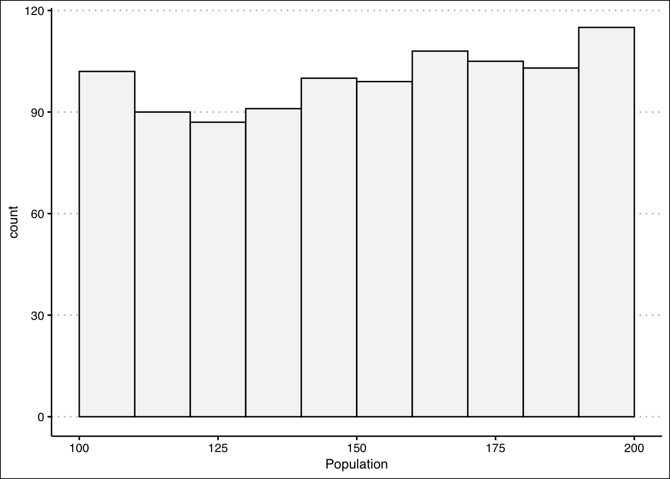
- Create a for loop (with 1000 iterations) that takes a sample of 10 points from population, calculate the mean, and then store the result in a vector called SampleMeans. Calculate the mean of the SampleMeans object. How does this mean compare to PopMean? How does the standard deviation compare to PopSD?
Answer
Now let’s create a for loop that allows us to sample the population several times. In fact, we will sample the population 1000 times and record the mean of the samples.
nrep<-1000
SampleMeans<-c()
for (i in 1:nrep){
  x<-sample(Population,10,replace=T)
  SampleMeans<-c(SampleMeans,mean(x))
}
Now we can calculate the mean of the sample means in R:
mean(SampleMeans)[1] 151.4461Note that the mean is very close to PopMean. In the limit (that is if we take many more samples), these two values are equal to each other. Now let’s calculate the standard deviation of the sample means.
sd(SampleMeans)[1] 9.364747As you can see, the standard deviation is much lower. In fact, if we take PopSD and divide by 10 (the size of the sample), we should get close to the standard deviation of the sample means.
PopSD/sqrt(10)[1] 9.172602- Create a histogram for the sample means. Is the distribution uniform? Is it normal? What is the probability that the sample mean is between 140 and 160?
Answer
To create the histogram we use the geom_histogram() function once more:
ggplot() +
  geom_histogram(aes(SampleMeans),bg="#F5F5F5",
                 col="black", bins=10) +
  theme_clean()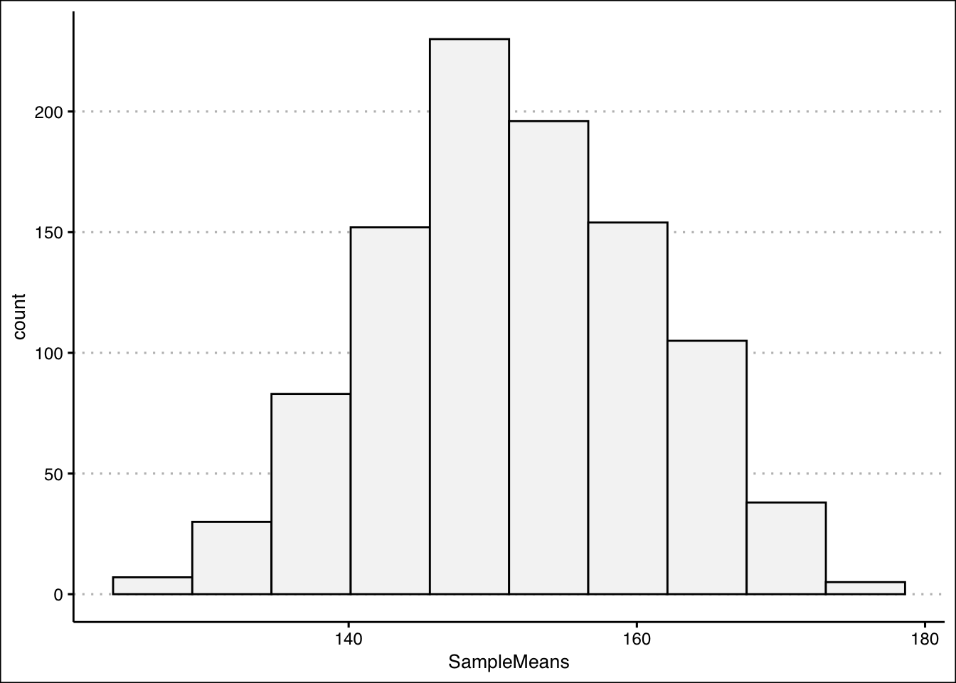
The distribution looks normal. To be clear, if the population follows a uniform distribution, we have shown that the distribution of the sample means is normal with a mean equal to the population mean and a smaller standard deviation. We can use the distribution of the sample means to calculate the desired probability. Noting the the distribution is normal:
pnorm(160,mean(SampleMeans),sd(SampleMeans))-pnorm(140,mean(SampleMeans),sd(SampleMeans))[1] 0.708682There is a \(70.87\)% probability that the sample mean is between \(140\) and \(160\).
Exercise 2
- A random sample of \(n=100\) is taken from a population with mean \(\mu=80\) and standard deviation \(\sigma=14\). Calculate the expected value and standard error for the sampling distribution of the sampling means. What is the probability that the sample mean falls between \(77\) and \(85\)?
Answer
The expected value is \(80\) since it is equal to the mean of the population. The standard error is \(1.4\). The probability is \(98.38\)%.
We can use R as a calculator to find the standard error.
14/sqrt(100)[1] 1.4We can use pnorm() to find the probability:
pnorm(85,80,1.4)-pnorm(77,80,1.4)[1] 0.9837602- Assume that miles-per-gallons of combustion cars are normally distributed with mean of \(33.8\) and standard deviation of \(3.5\). What is the probability that the mean mpg of four randomly selected cars is more than \(35\)? What is the probability that all four selected cars have mpg greater than \(35\)?
Answer
The probabilities are \(24.66\)% and \(1.8\)%.
For the first probability we can use a sample size of \(4\) and use the standard error in the pnorm() function.
pnorm(35,33.8,3.5/sqrt(4),lower.tail = F)[1] 0.2464466For the second probability we can first calculate the probability that a randomly selected car has mpg greater than \(35\). In R:
(p35<-pnorm(35,33.8,3.5,lower.tail = F))[1] 0.365853Since draws are independent we get:
p35^4[1] 0.01791539Exercise 3
- A random sample of \(n=200\) is taken from a population with a proportion of \(p=0.75\). Calculate the expected value and standard error of the proportion sampling distribution. What is the probability that the sample proportion is between \(0.7\) and \(0.8\)?
Answer
The expected value is \(0.75\), the same as the population. The standard error is \(\sqrt{p(1-p)/n}=0.03\). The probability for a sample of \(200\) is \(0.8975\).
The standard error is given by:
sqrt(0.75*0.25/200)[1] 0.03061862In R we can use the pnorm() function one more time to find the probability.
pnorm(0.8,0.75,sqrt(0.75*0.25/200))-pnorm(0.7,0.75,sqrt(0.75*0.25/200))[1] 0.89752962.Twenty-three percent of employees at a fintech firm work from home. If we take a sample of 50 employees, what is the probability that more than 20% of them are working from home? What if the sample increases to 200? Why does the probability change?
Answer
The probability with a sample of \(50\) is \(69.29\)%. When the sample is \(200\) the probability is \(84.33\)%. As the sample size increases the standard error goes down. This means that the distribution of the sample proportions gets tighter and there is more area to the right of \(\bar{p}=0.2\).
In R we can use the pnorm() function one more time with a mean of \(0.2\) and \(n=50\).
pnorm(0.2,0.23,sqrt(0.23*0.77/50),lower.tail = F)[1] 0.6928964Updating the code so that \(n=200\) yields:
pnorm(0.2,0.23,sqrt(0.23*0.77/200),lower.tail = F)[1] 0.8433098Exercise 4
- A production process for energy drinks is being evaluated. The machine that fills the cans is calibrated so that each can has \(350\)ml of drink with a standard deviation of \(10\)ml. Every hour, ten cans are sampled and the average amount of drink is recorded (see table below). Is the machine working properly?
| 1 | 2 | 3 | 4 | 5 | 6 | 7 | 8 |
|---|---|---|---|---|---|---|---|
| \(\bar{x}=310\) | \(\bar{x}=315\) | \(\bar{x}=325\) | \(\bar{x}=330\) | \(\bar{x}=328\) | \(\bar{x}=347\) | \(\bar{x}=339\) | \(\bar{x}=350\) |
Answer
The process seems to be out of control. In the early samples, the machine is not filling the cans with enough drink. Although, in the later periods the machine reverts back to the expected performance, it seems unlikely that it will remain functioning correctly.
Let’s start by calculating the upper and lower limits in R.
dataEx1<-c(310,315,325,330,328,347,339,350)
ulEx1<-350+3*(10/sqrt(10))
llEx1<-350-3*(10/sqrt(10))
We can graph the samples and the limits to determine the stability of the production process.
ggplot() +
  geom_point(aes(y=dataEx1, x=1:8), pch=21,
             bg="blue", alpha=0.3)+
  geom_hline(yintercept = ulEx1, col="red", lty=2) +
  geom_hline(yintercept = llEx1, col="red",lty=2) +
  theme_clean() +
  labs(y="Volume (ml)", x="Sample")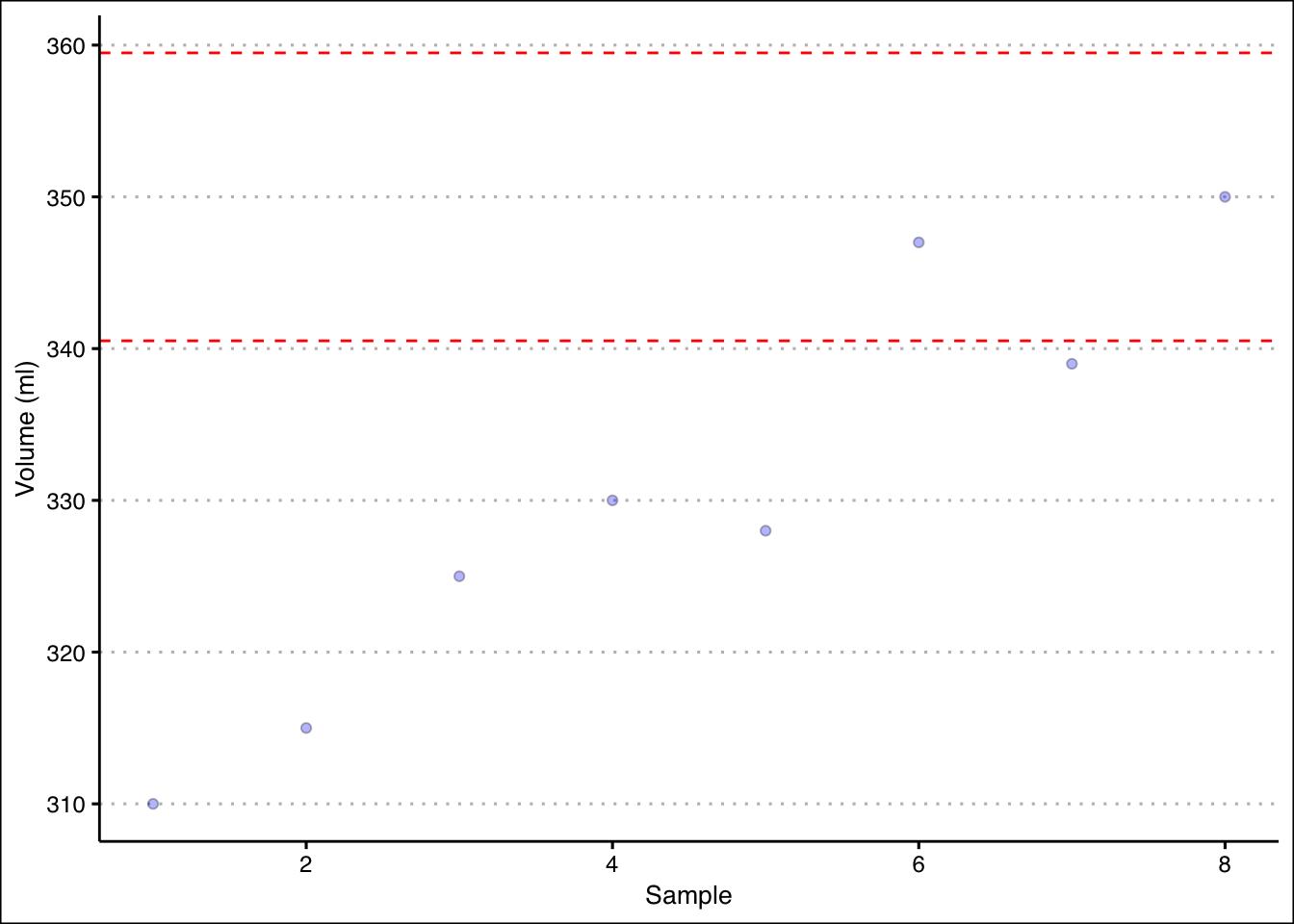
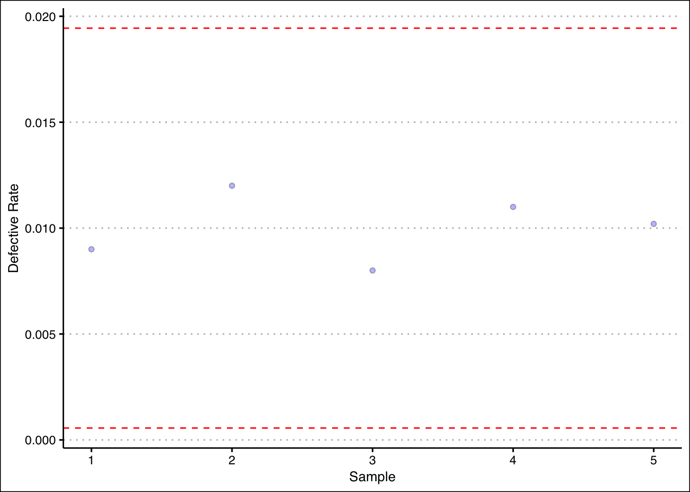
- The production of Good Guy dolls has a \(1\)% defective rate. A quality inspector takes five samples of size \(1000\). The proportions are shown in the table below. Is the production process under control?
| 1 | 2 | 3 | 4 | 5 |
|---|---|---|---|---|
| \(\bar{p}=0.009\) | \(\bar{p}=0.012\) | \(\bar{p}=0.008\) | \(\bar{p}=0.011\) | \(\bar{p}=0.0102\) |
Answer
Good Dolls production looks good. All proportions fall between three standard errors of the mean.
Once more we can calculate upper and lower limits for the proportions.
dataEx2<-c(0.009,0.012,0.008,0.011,0.0102)
ulEx2<-0.01+3*sqrt(0.01*0.99/1000)
llEx2<-0.01-3*sqrt(0.01*0.99/1000)
Graphing the results in R we can observe the production process and the sample proportions.
ggplot() +
  geom_point(aes(y=dataEx2, x=1:5), pch=21,
             bg="blue", alpha=0.3)+
  geom_hline(yintercept = ulEx2, col="red", lty=2) +
  geom_hline(yintercept = llEx2, col="red",lty=2) +
  theme_clean() +
  labs(y="Defective Rate", x="Sample")